Downloaded 1,295 times


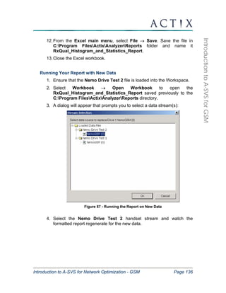
![Introduction to A-SVS for Network Optimization - GSM Page 50
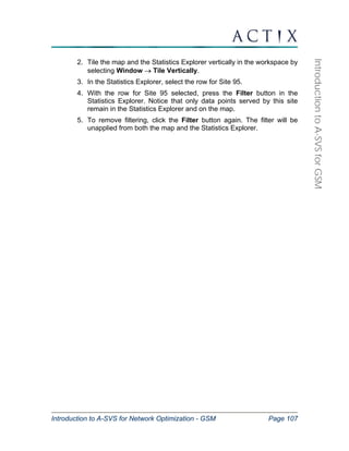
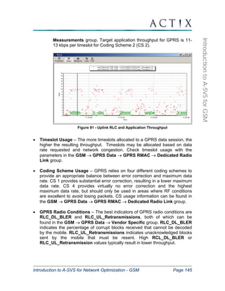
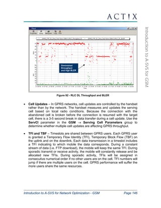
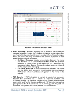
Introduction to A-SVS for GSM
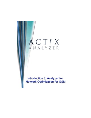
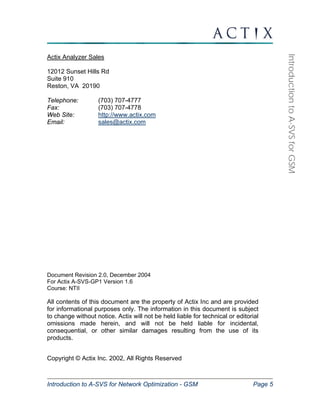
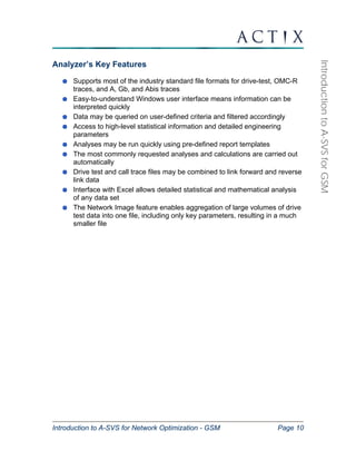
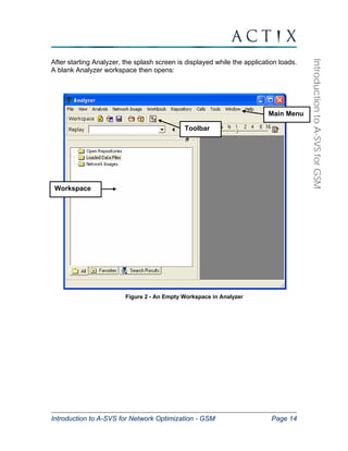
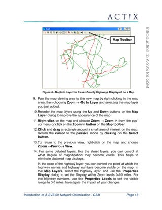
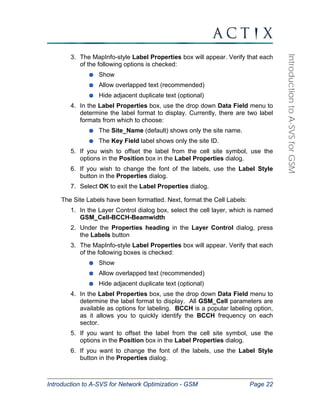
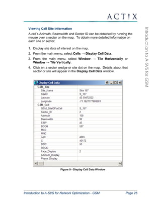
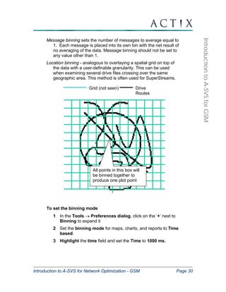
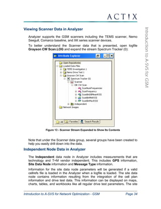
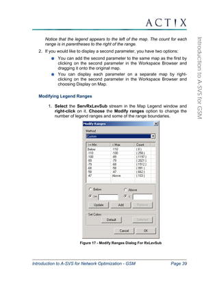
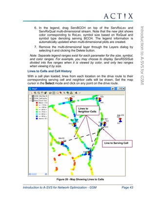
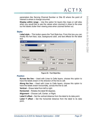
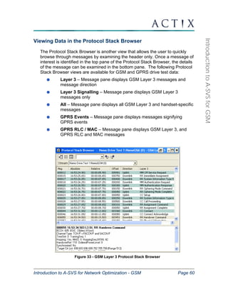
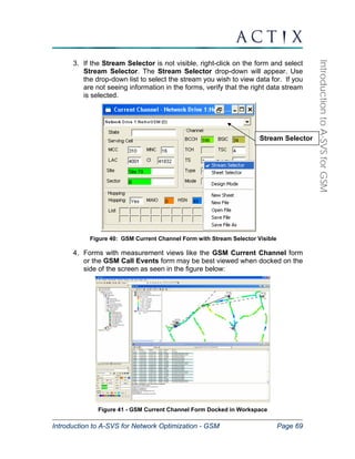
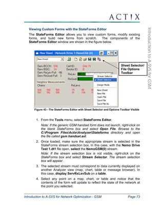
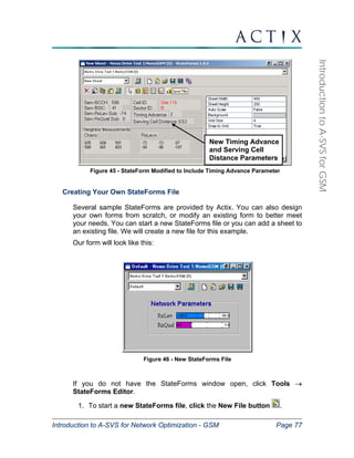
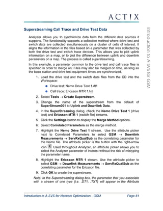
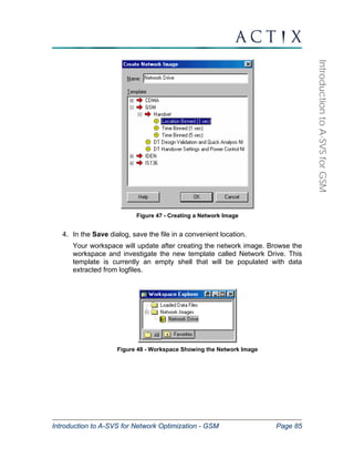
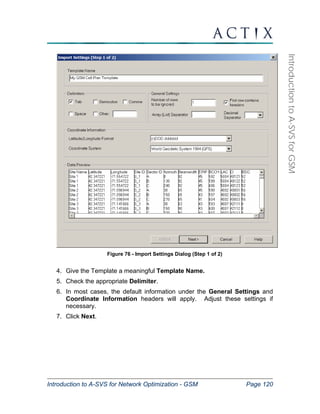
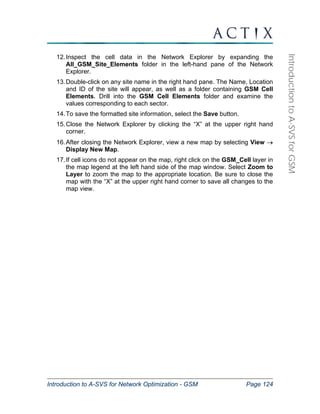
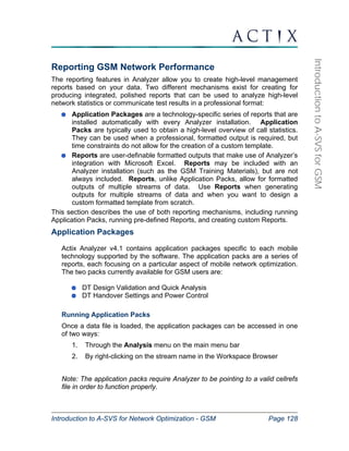
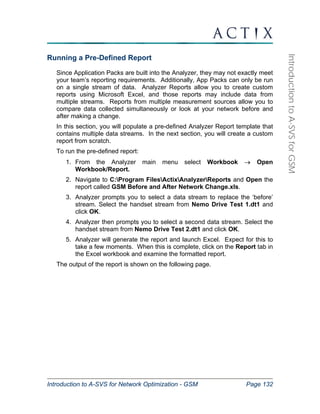
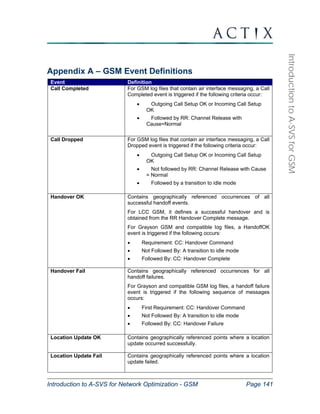
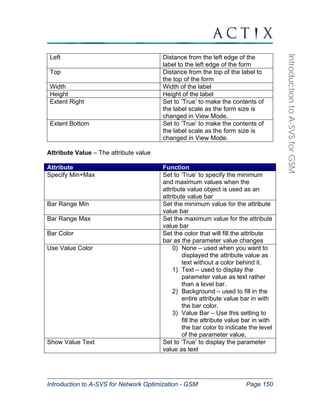
to each corner of the desired region to filter and click the mouse
once. To finish drawing the polygon, double-click near the starting
point to establish a line between the last point and the first point.
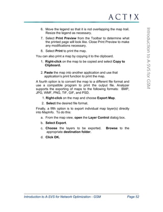
3. Draw any other polygons, as needed.
4. To filter data, click the down-arrow next to Filter and select either
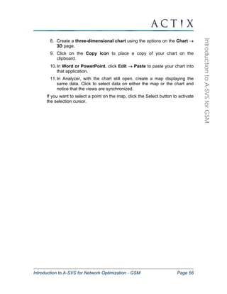
Include or Exclude. “Include” is the default filter. [Note: Any
additional attributes that are dragged onto a map using regional
filtering will also be filtered].
5. To remove the filter, select Remove All from the map toolbar. This
will delete all existing region filters in that map. Region filters in other
map windows are unaffected.
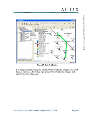
Figure 27: Region Filtering using "Include"](https://image.slidesharecdn.com/actixanalyzertrainingmanualforgsm-141019060755-conversion-gate02/85/Actix-analyzer-training_manual_for_gsm-50-320.jpg)
![Introduction to A-SVS for Network Optimization - GSM Page 64
Introduction to A-SVS for GSM
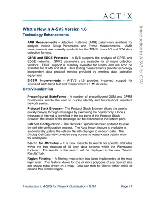
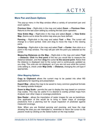
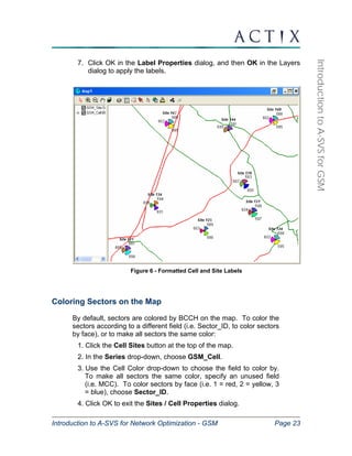
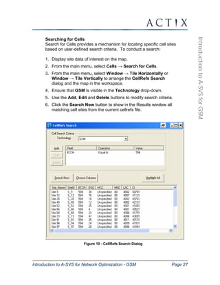
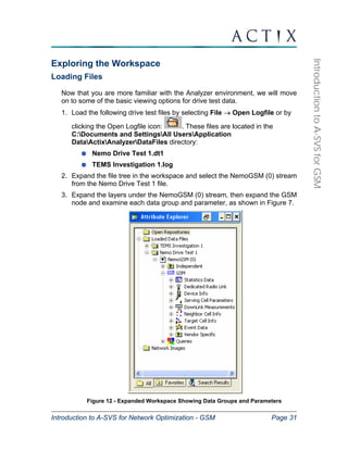
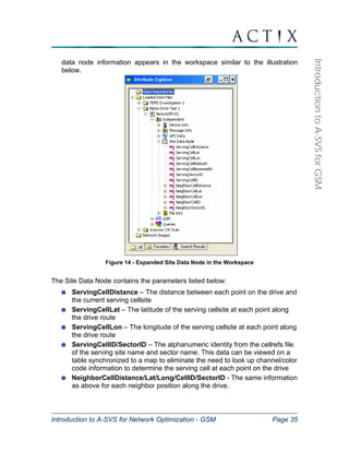
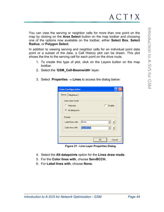
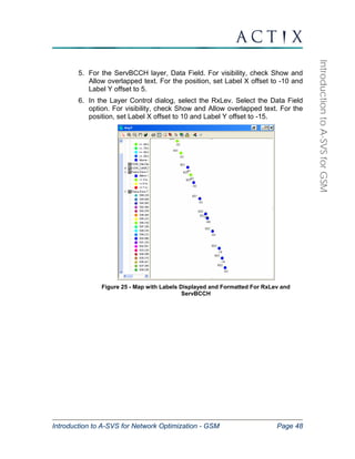
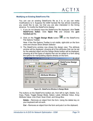
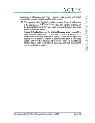
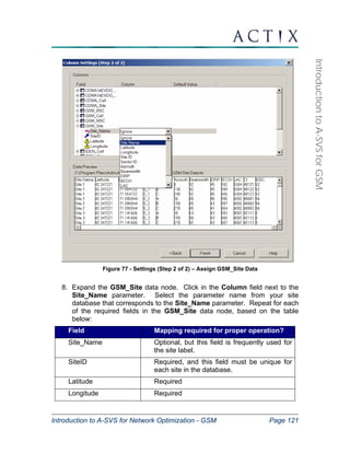
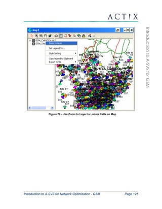
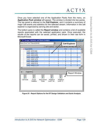
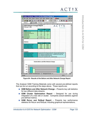
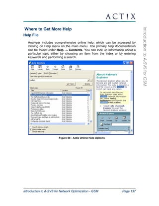
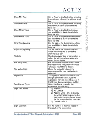
it appears in the Attribute Explorer. Press “Enter” to reactivate
the page.
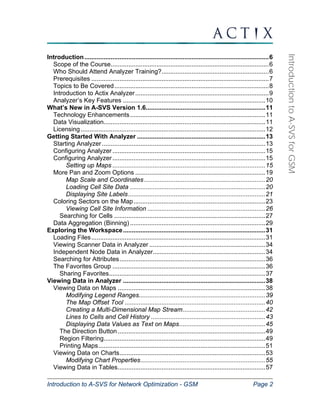
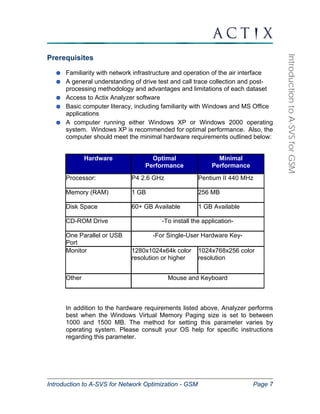
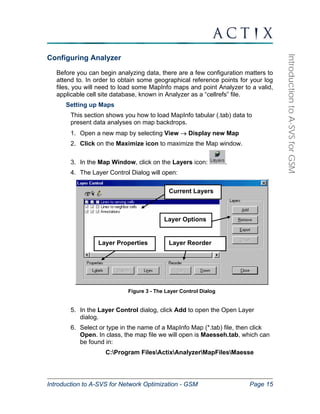
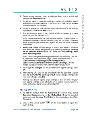
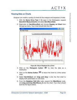
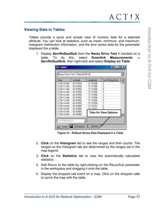
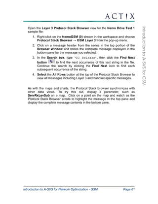
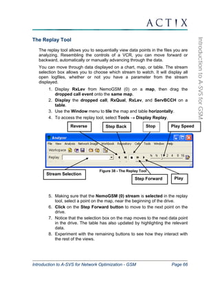
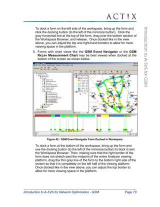
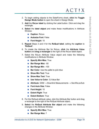
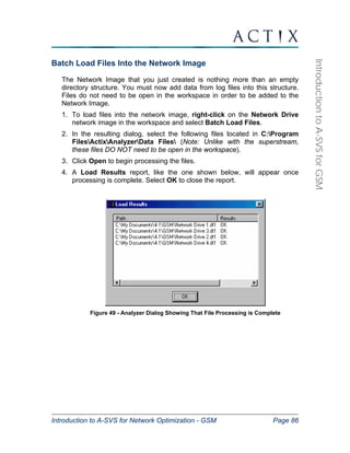
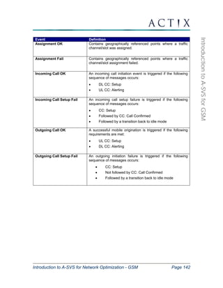
4. Select “Click Here” on the Binning line to enter the Preferences
dialog. Change the binning settings to:
a. Binning Mode = Location
b. Projection = Default (meters) [Scroll up from default entry
to find this option]
c. X size = 50
d. Y size = 50
e. Unit = Meters
Figure 36: Setting the Binning for Delta Plot Creation
5. Select the “Before” stream
6. Select the “After” stream
7. Enter an alternative name for the delta stream (if desired).
Press “Enter” when done to reactivate the task page
8. Click the “Create Delta Plot” button
The delta value is calculated by subtracting the “After” stream from the
“Before” stream. Once the delta plot has been created, a map will appear
containing the two original streams and the delta value between the two
streams.](https://image.slidesharecdn.com/actixanalyzertrainingmanualforgsm-141019060755-conversion-gate02/85/Actix-analyzer-training_manual_for_gsm-64-320.jpg)
![Introduction to A-SVS for Network Optimization - GSM Page 91
Introduction to A-SVS for GSM
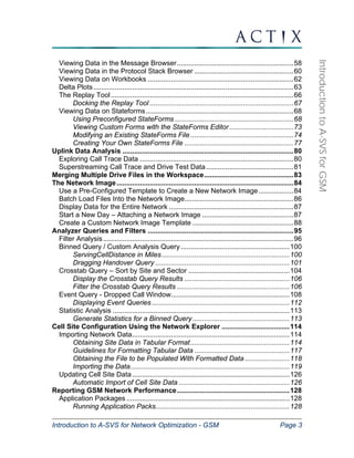
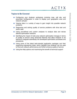
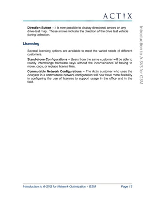
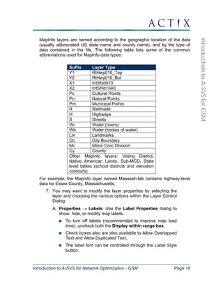
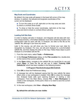
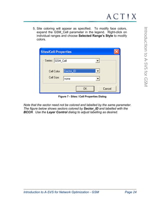
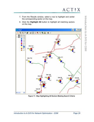
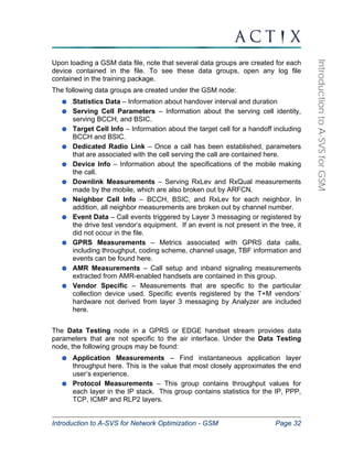
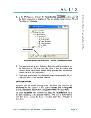
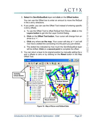
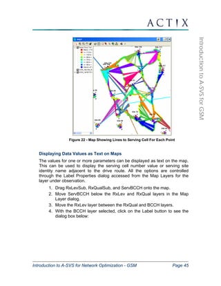
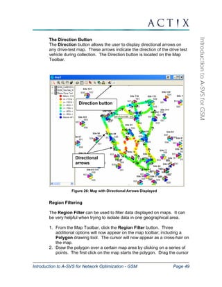
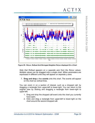
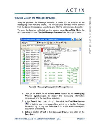
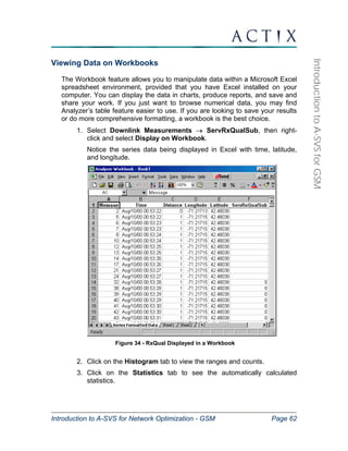
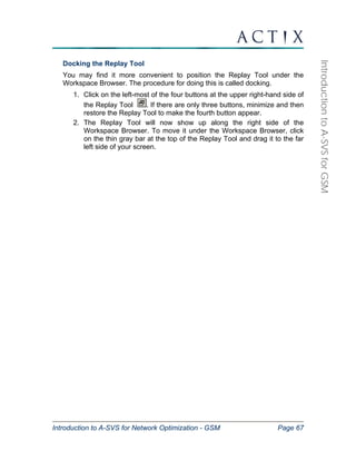
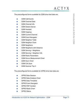
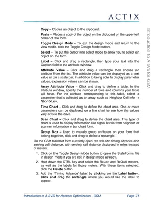
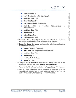
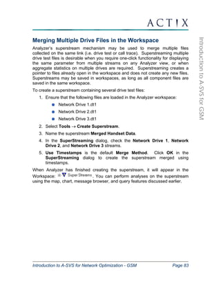
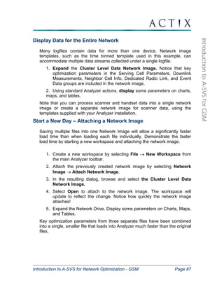
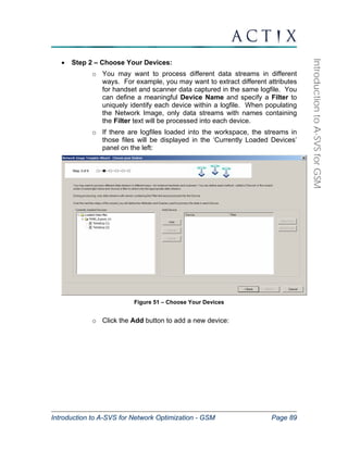
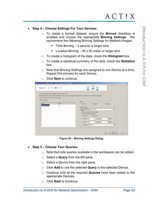
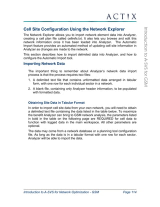
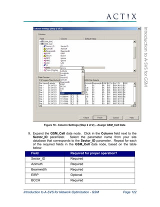
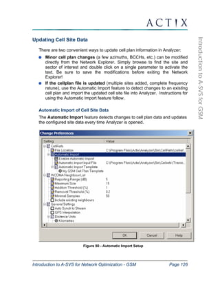
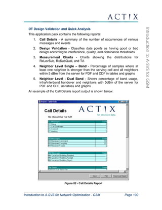
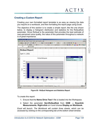
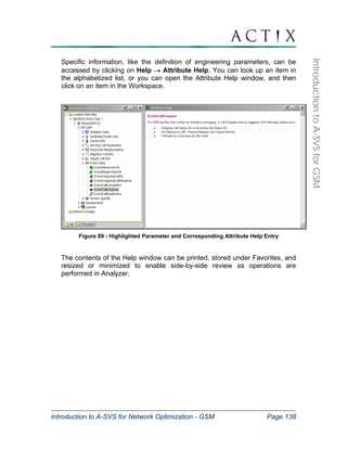
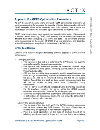
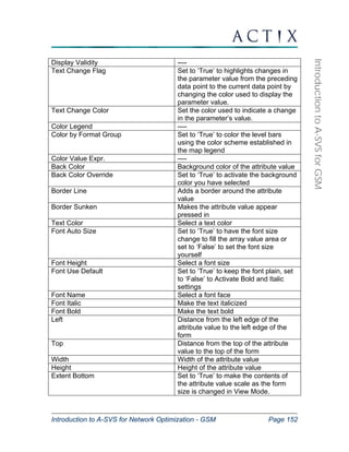
• Step 3 – Choose Your Attributes:
o Select a Device from the panel on the right, and then use the
Add button to select the required attributes from the Attribute
Picker panel on the left.
o If you select an array attribute (i.e.
ScanSortSigLevel_by_SigLevel[]), a dialog will prompt you for
the range of indices. Enter the start and end values and click
OK.
o In addition to standard analysis parameters, we recommend
adding the Independent → FileName parameter to each
Device in a Network Image. FileName can be used to trace
data points in the Network Image to the original source file. This
method is used to perform detailed analysis on problems
spotted in the high level Network Image.
o Attributes are assigned to one Device at a time. To duplicate
the attributes selected for one Device into another Device,
select the Device with the required attributes and click Copy.
Then select the second Device and click Paste.
o Once you have added all required attributes, click Next to
continue.
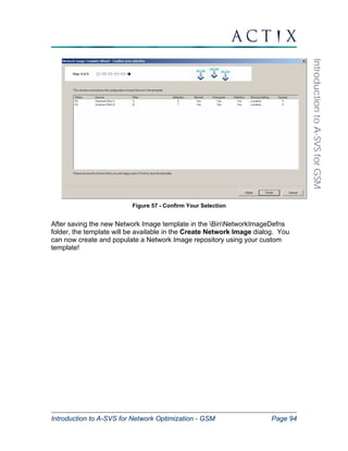
Figure 54 – Choose Your Attributes](https://image.slidesharecdn.com/actixanalyzertrainingmanualforgsm-141019060755-conversion-gate02/85/Actix-analyzer-training_manual_for_gsm-91-320.jpg)
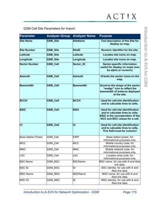
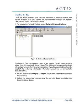
![Introduction to A-SVS for Network Optimization - GSM Page 102
Introduction to A-SVS for GSM
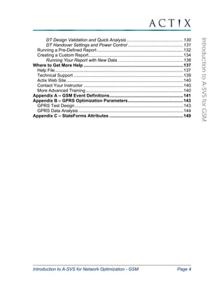
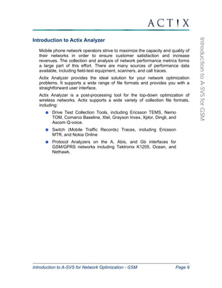
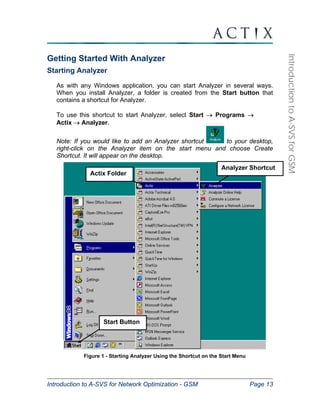
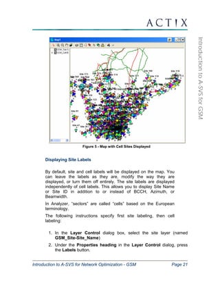
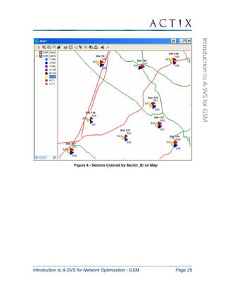
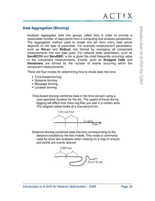
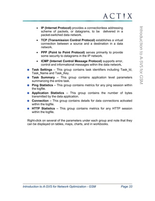
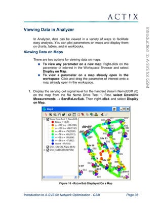
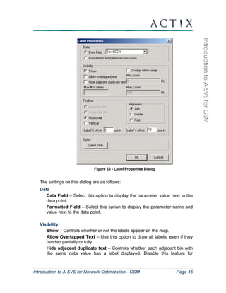
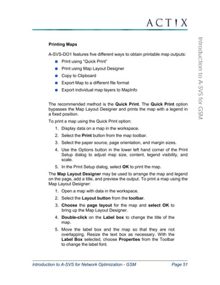
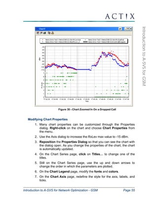
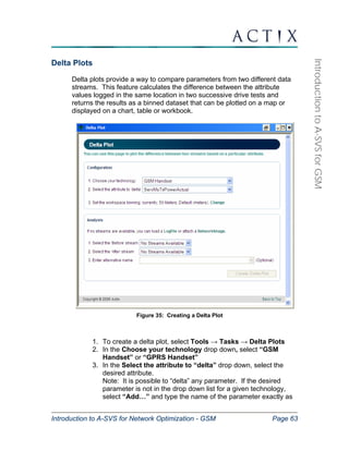
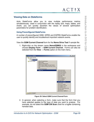
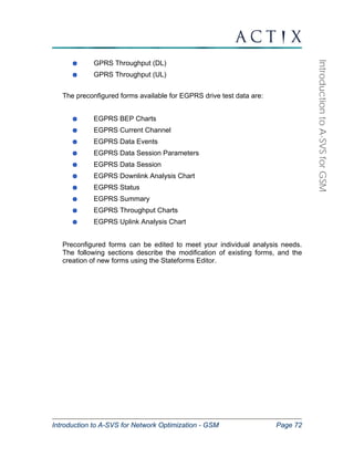
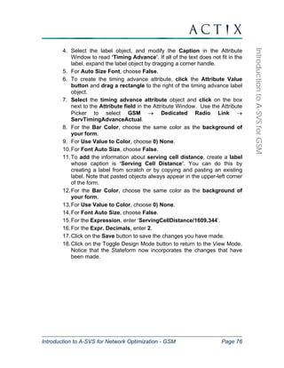
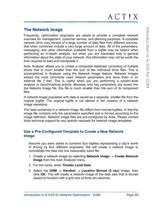
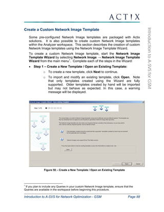
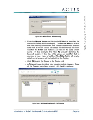
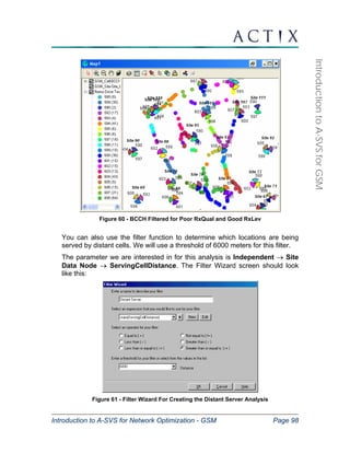
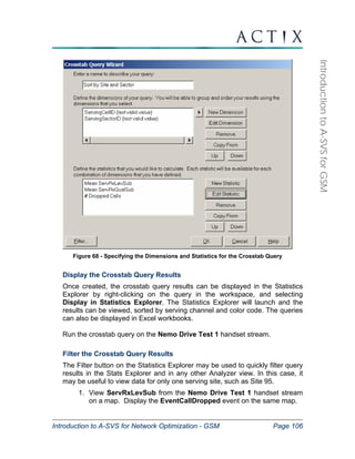
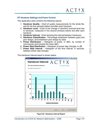
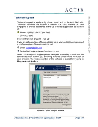
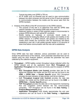
We will create a custom parameter that identifies locations where the RxLev
for any neighbor is more than 8 dB greater than the RxLev of the serving
sector.
The Expression is: (array_max(NborRxLev[])-8)>ServRxLevSub
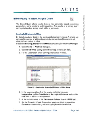
4. In the Expression Builder, type ‘(‘.
5. From the available functions, double-click on the array_max function. This
function will parse an array and select the largest value in it.
6. Click to select the <<attribute[]>> placeholder in the Expression Builder.
In the Parameters pane select GSM → Neighbor Cell Info → NborRxLev
and double-click on it to add it to the expression.
7. At the end of the text in the Expression Builder, type in ‘-8)>’.
8. In the attribute pane, go to GSM → Downlink Measurements →
ServRxLevSub and double-click to add it to the expression.
9. Set the Format to Boolean. The easiest way to do this is to select the
Format drop down dialog and start typing Boolean in the window.
10. Click OK to create the query.
11. Click OK again to close the Analysis Manager.
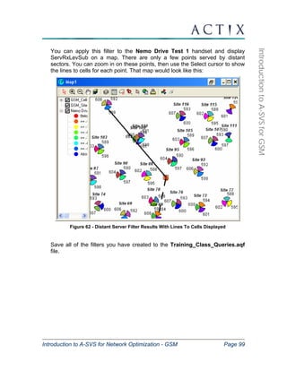
12. The query will appear in a new Queries group under every data stream in
the workspace. Under the Nemo Drive Test 1 handset stream, expand
the Queries → Binned Queries group.
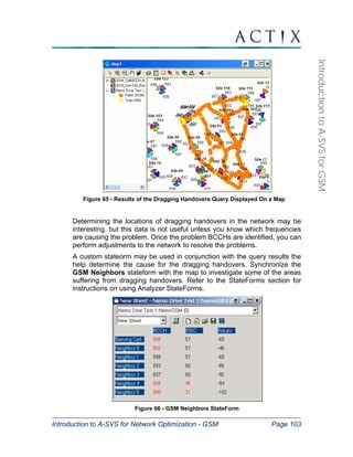
13. Right-click on the Dragging Handovers ? query and choose Display on
Map to display the query results on a map.](https://image.slidesharecdn.com/actixanalyzertrainingmanualforgsm-141019060755-conversion-gate02/85/Actix-analyzer-training_manual_for_gsm-102-320.jpg)
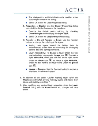
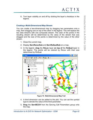
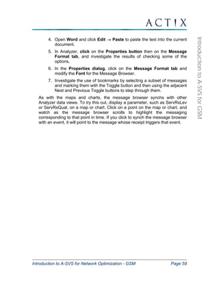
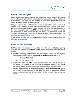
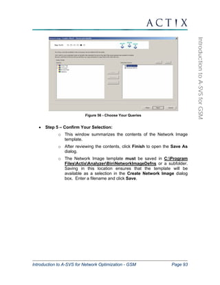
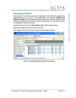
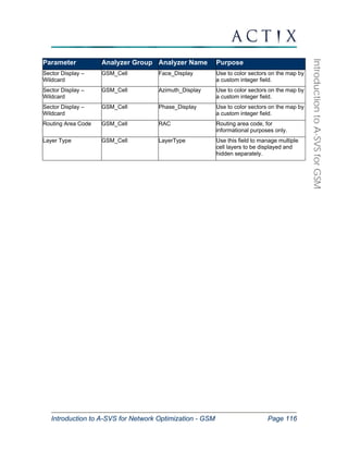
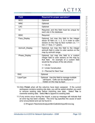
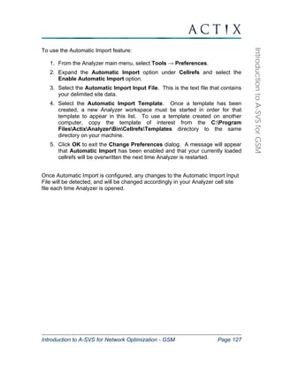
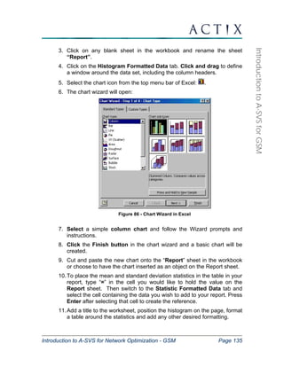
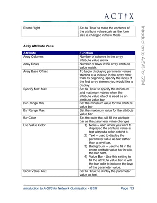
![Expression Method to Calculate
State(ServingSectorID) Last Value
State(ServBCCH) Last Value
State(ServBSIC) Last Value
ServRXLev Mean
ServRxQual Mean
State(NborBCCH[0]) Last Value
NborRxLev[0] Mean
Introduction to A-SVS for Network Optimization - GSM Page 111
Introduction to A-SVS for GSM
Figure 72 - Expression Builder for the Event Query
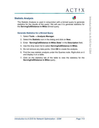
13. In the Statistic window, select the method to calculate the statistic. In
this case, select Last Value. Click OK when finished with the Statistic
window.
14. Repeat steps 7 through 13 above to define the following statistics
(choose an appropriate name for each one). The statistics that do not
require the use of the State() function can be picked using the
Attribute Chooser instead of the Expression Builder.
15. Once completed, click OK in all other active dialogs to complete the
query.](https://image.slidesharecdn.com/actixanalyzertrainingmanualforgsm-141019060755-conversion-gate02/85/Actix-analyzer-training_manual_for_gsm-111-320.jpg)


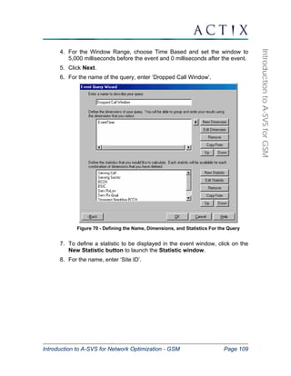
This document provides an introduction to using Actix Analyzer software for analyzing GSM network performance. It covers loading and viewing drive test and other radio network data, performing queries and filters on the data, configuring cell sites and networks, and generating reports. Key features discussed include mapping cells and drive test data, binning and aggregating data, exploring data on charts and tables, and using preconfigured applications and reports for common analysis tasks.


