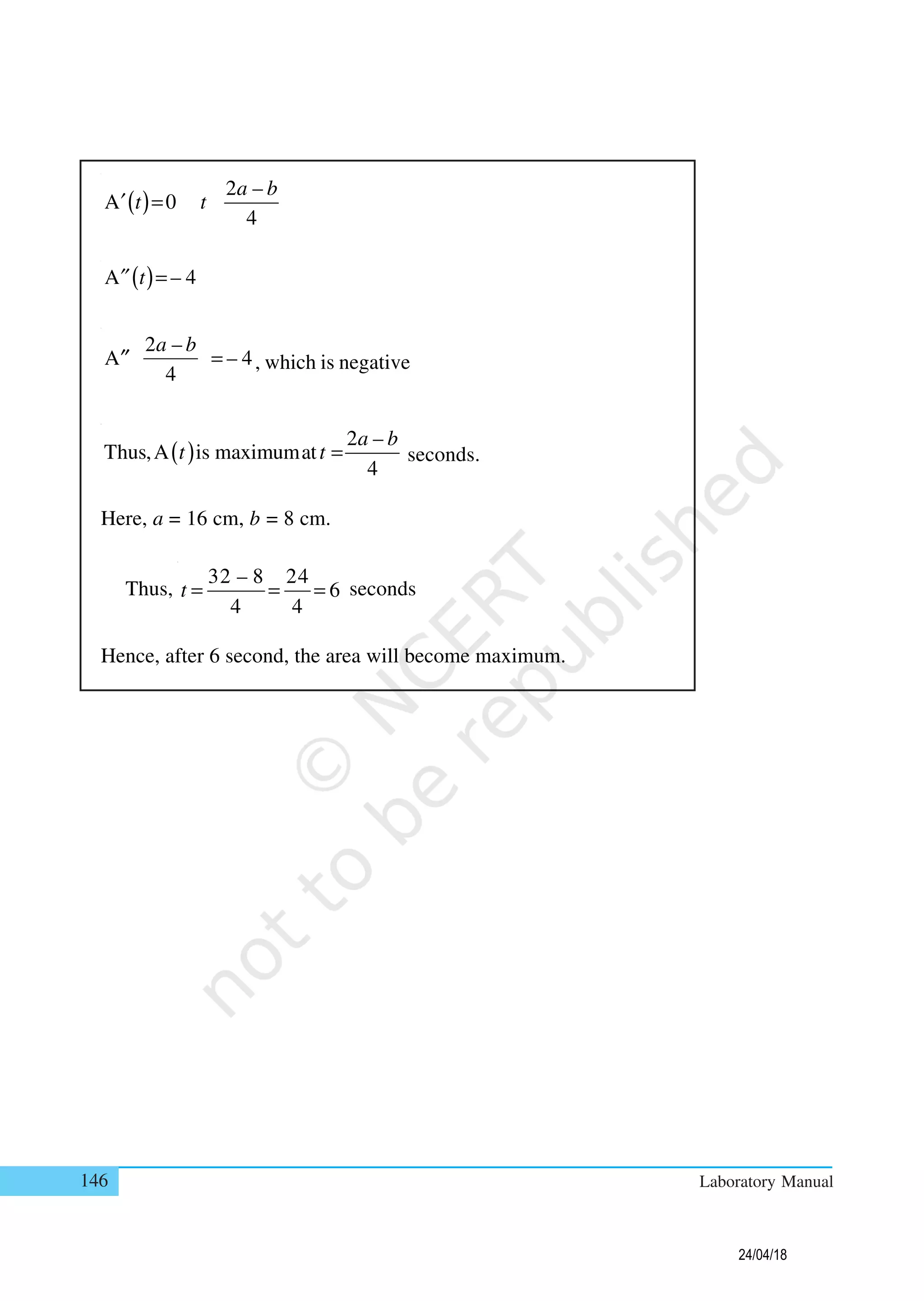
1. The document describes constructing a graph to demonstrate absolute maximum and minimum values of a function. 2. A chart paper is marked with x and y axes and the function f(x) = (4x^2 - 9)(x^2 - 1) is graphed over the interval [-2, 2] by plotting ordered pairs and connecting the points. 3. The graph illustrates the absolute maximum and minimum values of the function over the given interval.

1. METHOD OF CONSTRUCTION
1. Take a cardboard of a convenient size and paste a white paper on it.
2. Take two wires of convenient size and fix them on the white paper pasted on
the plywood to represent x-axis and y-axis (see Fig. 11).
3. Take a piece of wire of 15 cm length and bend it in the shape of a curve and
fix it on the plywood as shown in the figure.
OBJECTIVE MATERIALREQUIRED
To verify Rolle’s Theorem. A piece of plywood, wires of
different lengths, white paper,
sketch pen.
Activity 11
4. Take two straight wires of the same length and fix them in such way that
they are perpendicular to x-axis at the points A and B and meeting the curve
at the points C and D (see Fig.11).
24/04/18

2. 128 Laboratory Manual
DEMONSTRATION
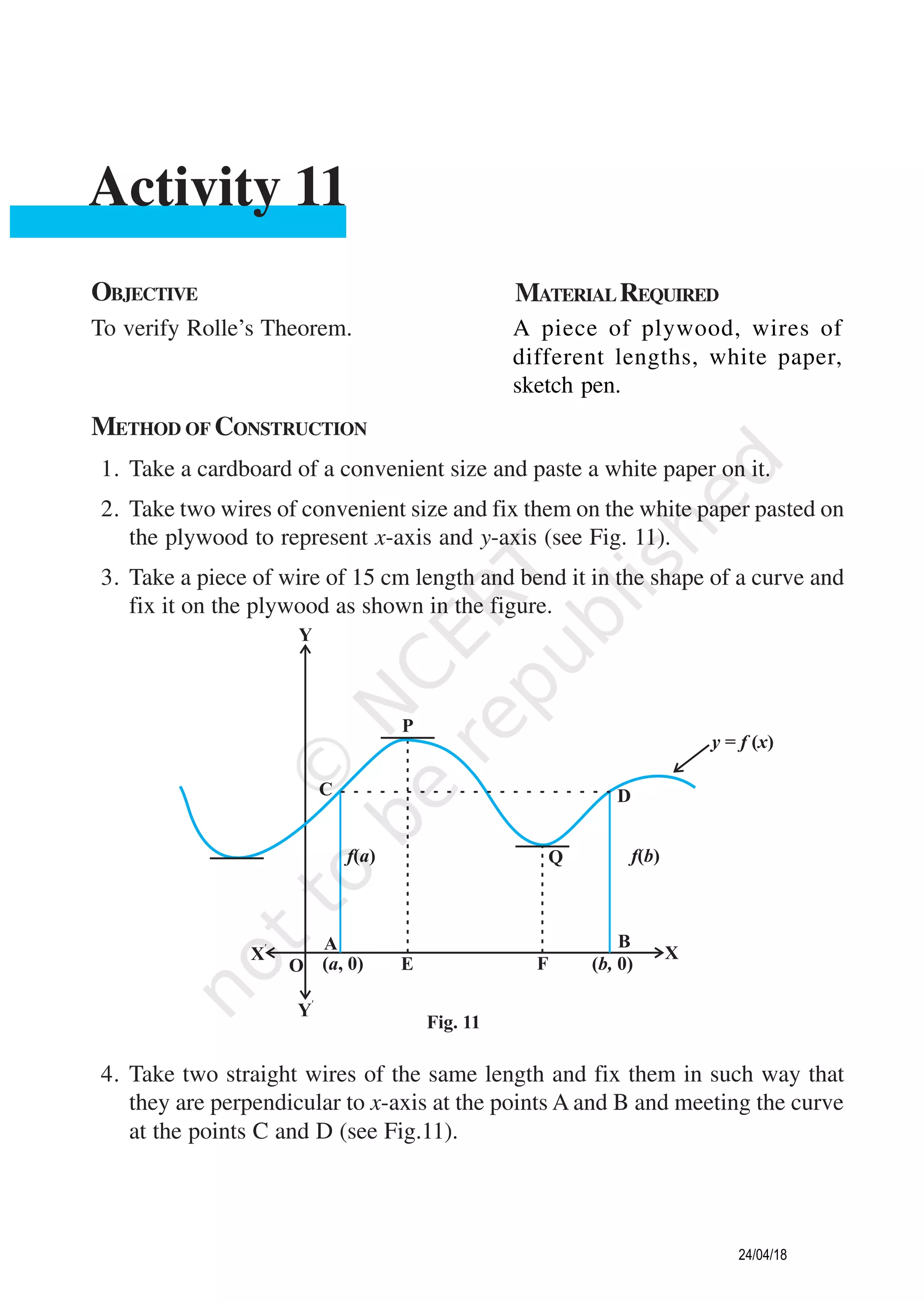
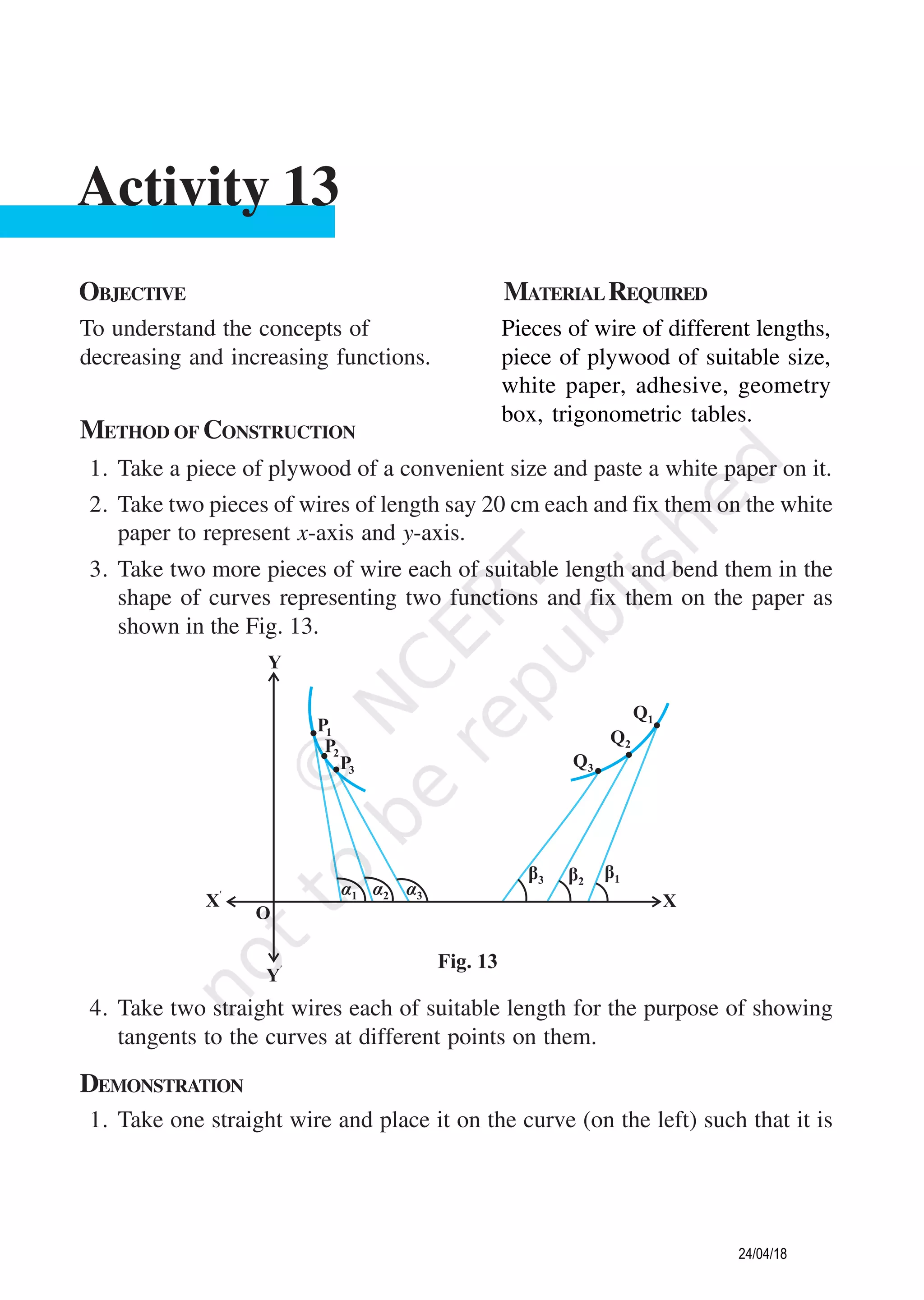
1. In the figure, let the curve represent the function y = f (x). Let OA = a units
and OB = b units.
2. The coordinates of the points A and B are (a, 0) and (b, 0), respectively.
3. There is no break in the curve in the interval [a, b]. So, the function f is
continuous on [a, b].
4. The curve is smooth between x = a and x = b which means that at each point,
a tangent can be drawn which in turn gives that the function f is differentiable
in the interval (a, b).
5. As the wires at A and B are of equal lengths, i.e., AC = BD, so f (a) = f (b).
6. In view of steps (3), (4) and (5), conditions of Rolle’s theorem are satisfied.
From Fig.11, we observe that tangents at P as well as Q are parallel to
x-axis, therefore, f ′ (x) at P and also at Q are zero.
Thus, there exists at least one value c of x in (a,b) such that f ′ (c) = 0.
Hence, the Rolle's theorem is verified.
OBSERVATION
From Fig. 11.
a = ______________, b = _____________
f (a) = ____________, f (b) = _________ Is f (a) = f (b) ? (Yes/No)
Slope of tangent at P = __________, so, f (x) (at P) =
APPLICATION
This theorem may be used to find the roots of an equation.
24/04/18

3. METHOD OF CONSTRUCTION
1. Take a piece of plywood and paste a white paper on it.
2. Take two wires of convenient size and fix them on the white paper pasted on
the plywood to represent x-axis and y-axis (see Fig. 12).
3. Take a piece of wire of about 10 cm length and bend it in the shape of a
curve as shown in the figure. Fix this curved wire on the white paper pasted
on the plywood.
OBJECTIVE MATERIAL REQUIRED
To verify Lagrange’s Mean Value
Theorem.
A piece of plywood, wires, white
paper, sketch pens, wires.
Activity 12
24/04/18

4. 130 Laboratory Manual
4. Take two straight wires of lengths 10 cm and 13 cm and fix them at two
different points of the curve parallel to y-axis and their feet touching the
x-axis. Join the two points, where the two vertical wires meet the curve,
using another wire.
5. Take one more wire of a suitable length and fix it in such a way that it is
tangential to the curve and is parallel to the wire joining the two points on
the curve (see Fig. 12).
DEMONSTRATION
1. Let the curve represent the function y = f (x). In the figure, let OA = a units
and OB = b units.
2. The coordinates of A and B are (a, 0) and (b, 0), respectively.
3. MN is a chord joining the points M (a, f (a) and N (b, f (b)).
4. PQ represents a tangent to the curve at the point R (c, f (c)), in the interval
(a, b).
5. ( )f c′ is the slope of the tangent PQ at x = c.
6.
( ) ( )–
–
f b f a
b a
is the slope of the chord MN.
7. MN is parallel to PQ, therefore, ( )f c′ =
( ) ( )–
–
f b f a
b a
. Thus, the
Langrange’s Mean Value Theorem is verified.
OBSERVATION
1. a = __________, b = ______________,
f (a) = ________, f (b)= ____________.
2. f (a) – f (b) = ________,
b – a = ________,
24/04/18

5. Mathematics 131
3.
( )– ( )
–
f b f a
b a
= ________ = Slope of MN.
4. Since PQ || MN ⇒ Slope of PQ = f ′(c) =
( ) ( )f a f a
b a
−
−
.
APPLICATION
Langrange’s Mean Value Theorem has significant applications in calculus.
For example this theorem is used to explain concavity of the graph.
24/04/18

6. METHOD OF CONSTRUCTION
1. Take a piece of plywood of a convenient size and paste a white paper on it.
2. Take two pieces of wires of length say 20 cm each and fix them on the white
paper to represent x-axis and y-axis.
3. Take two more pieces of wire each of suitable length and bend them in the
shape of curves representing two functions and fix them on the paper as
shown in the Fig. 13.
OBJECTIVE MATERIALREQUIRED
To understand the concepts of
decreasing and increasing functions.
Pieces of wire of different lengths,
piece of plywood of suitable size,
white paper, adhesive, geometry
box, trigonometric tables.
Activity 13
4. Take two straight wires each of suitable length for the purpose of showing
tangents to the curves at different points on them.
DEMONSTRATION
1. Take one straight wire and place it on the curve (on the left) such that it is
24/04/18

7. Mathematics 133
tangent to the curve at the point say P1
and making an angle α1
with the
positive direction of x-axis.
2. α1
is an obtuse angle, so tanα1
is negative, i.e., the slope of the tangent at P1
(derivative of the function at P1
) is negative.
3. Take another two points say P2
and P3
on the same curve, and make tangents,
using the same wire, at P2
and P3
making angles α2
and α3
, respectively with
the positive direction of x-axis.
4. Here again α2
and α3
are obtuse angles and therefore slopes of the tangents
tan α2
and tan α3
are both negative, i.e., derivatives of the function at P2
and
P3
are negative.
5. The function given by the curve (on the left) is a decreasing function.
6. On the curve (on the right), take three point Q1
, Q2
, Q3
, and using the other
straight wires, form tangents at each of these points making angles β1
, β2
,
β3
, respectively with the positive direction of x-axis, as shown in the figure.
β1
, β2
, β3
are all acute angles.
So, the derivatives of the function at these points are positive. Thus, the
function given by this curve (on the right) is an increasing function.
OBSERVATION
1. α1
= _______ , > 90° α2
= _______ > _______, α3
= _______> _______,
tan α1
= _______, (negative) tan α2
= _______, ( _______ ), tan α3
=
_______, ( _______). Thus the function is _______.
2. β1
= _______< 90°, β2
= _______, < _______, β3
= _______ , < _______
tan β1
= _______ , (positive), tan β2
= _______, ( _______ ), tan β3
=
_______( _______ ). Thus, the function is _______.
APPLICATION
This activity may be useful in explaining the concepts of decreasing and
increasing functions.
24/04/18

8. METHOD OF CONSTRUCTION
1. Take a piece of plywood of a convenient size and paste a white paper on it.
2. Take two pieces of wires each of length 40 cm and fix them on the paper on
plywood in the form of x-axis and y-axis.
3. Take another wire of suitable length and bend it in the shape of curve. Fix
this curved wire on the white paper pasted on plywood, as shown in Fig. 14.
OBJECTIVE MATERIALREQUIRED
To understand the concepts of local
maxima, local minima and point of
inflection.
A piece of plywood, wires,
adhesive, white paper.
Activity 14
24/04/18

9. Mathematics 135
4. Take five more wires each of length say 2 cm and fix them at the pointsA, C,
B, P and D as shown in figure.
DEMONSTRATION
1. In the figure, wires at the points A, B, C and D represent tangents to the
curve and are parallel to the axis. The slopes of tangents at these points are
zero, i.e., the value of the first derivative at these points is zero. The tangent
at P intersects the curve.
2. At the points A and B, sign of the first derivative changes from negative to
positive. So, they are the points of local minima.
3. At the point C and D, sign of the first derivative changes from positive to
negative. So, they are the points of local maxima.
4. At the point P, sign of first derivative does not change. So, it is a point of
inflection.
OBSERVATION
1. Sign of the slope of the tangent (first derivative) at a point on the curve to
the immediate left of A is _______.
2. Sign of the slope of the tangent (first derivative) at a point on the curve to
the immediate right of A is_______.
3. Sign of the first derivative at a point on the curve to immediate left
of B is _______.
4. Sign of the first derivative at a point on the curve to immediate right
of B is _______.
5. Sign of the first derivative at a point on the curve to immediate left
of C is _______.
6. Sign of the first derivative at a point on the curve to immediate right
of C is _______.
7. Sign of the first derivative at a point on the curve to immediate left
of D is _______.
24/04/18

10. 136 Laboratory Manual
8. Sign of the first derivative at a point on the curve to immediate right
of D is _______.
9. Sign of the first derivative at a point immediate left of P is _______ and
immediate right of P is_______.
10. A and B are points of local _______.
11. C and D are points of local _______.
12. P is a point of _______.
APPLICATION
1. This activity may help in explaining the concepts of points of local maxima,
local minima and inflection.
2. The concepts of maxima/minima are useful in problems of daily life such
as making of packages of maximum capacity at minimum cost.
24/04/18

11. OBJECTIVE MATERIALREQUIRED
To understand the concepts of
absolute maximum and minimum
values of a function in a given closed
interval through its graph.
Drawing board, white chart paper,
adhesive, geometry box, pencil and
eraser, sketch pens, ruler, calculator.
Activity 15
1 12
4
2
6
8
10
12
O
Y
X
2
2
4
3
2
1.27
16
20
14
18
22
1
2
3
2
2 1
X¢
Y¢
Fig 15
24/04/18

12. 138 Laboratory Manual
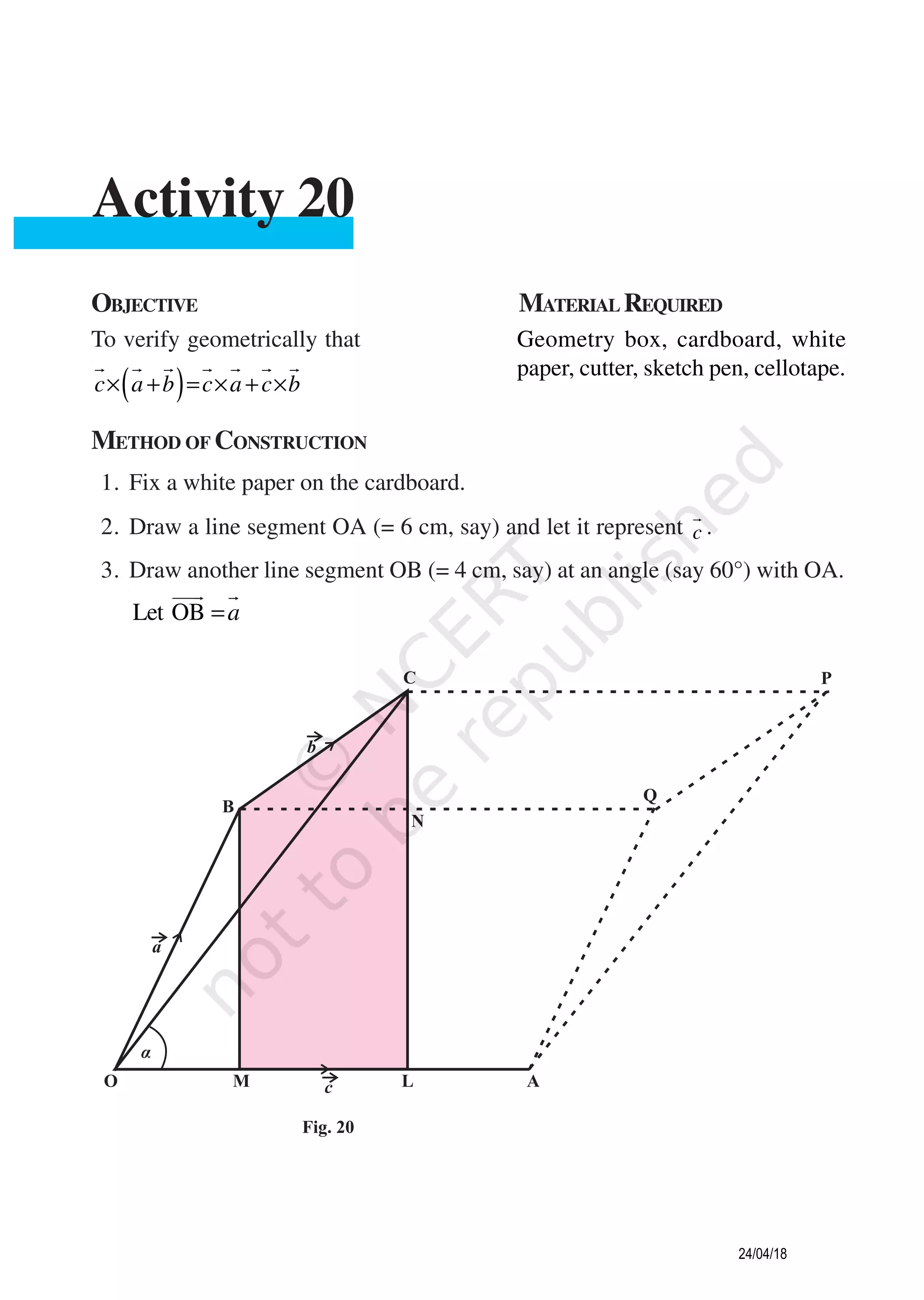
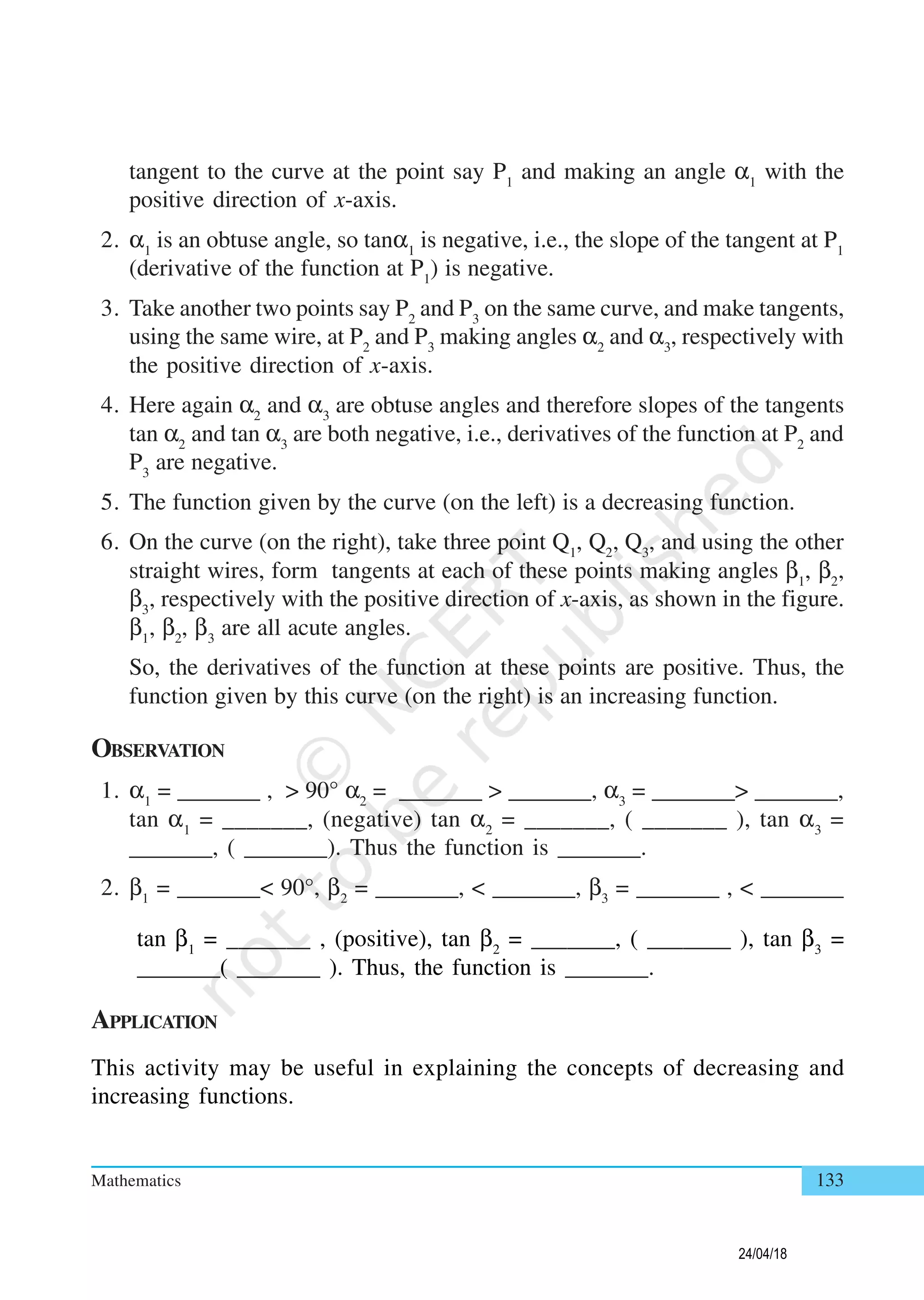
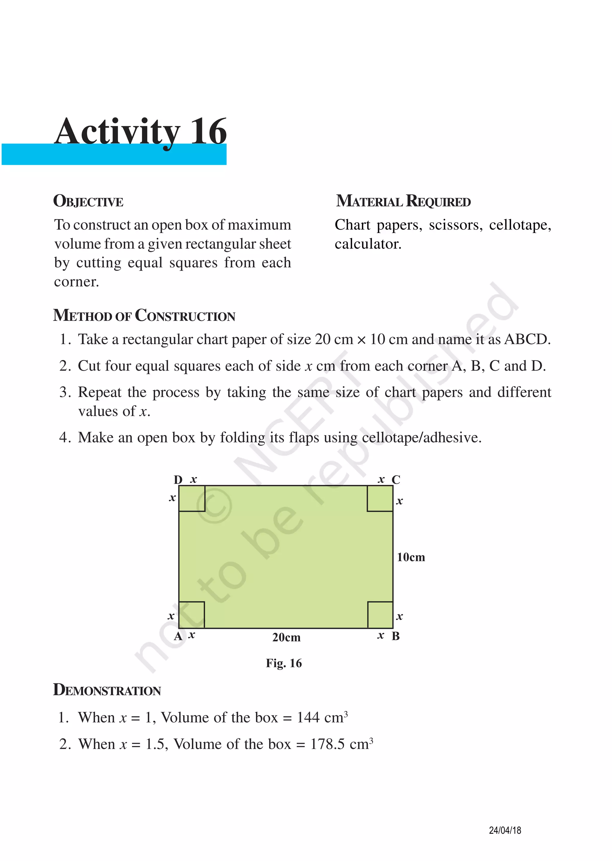
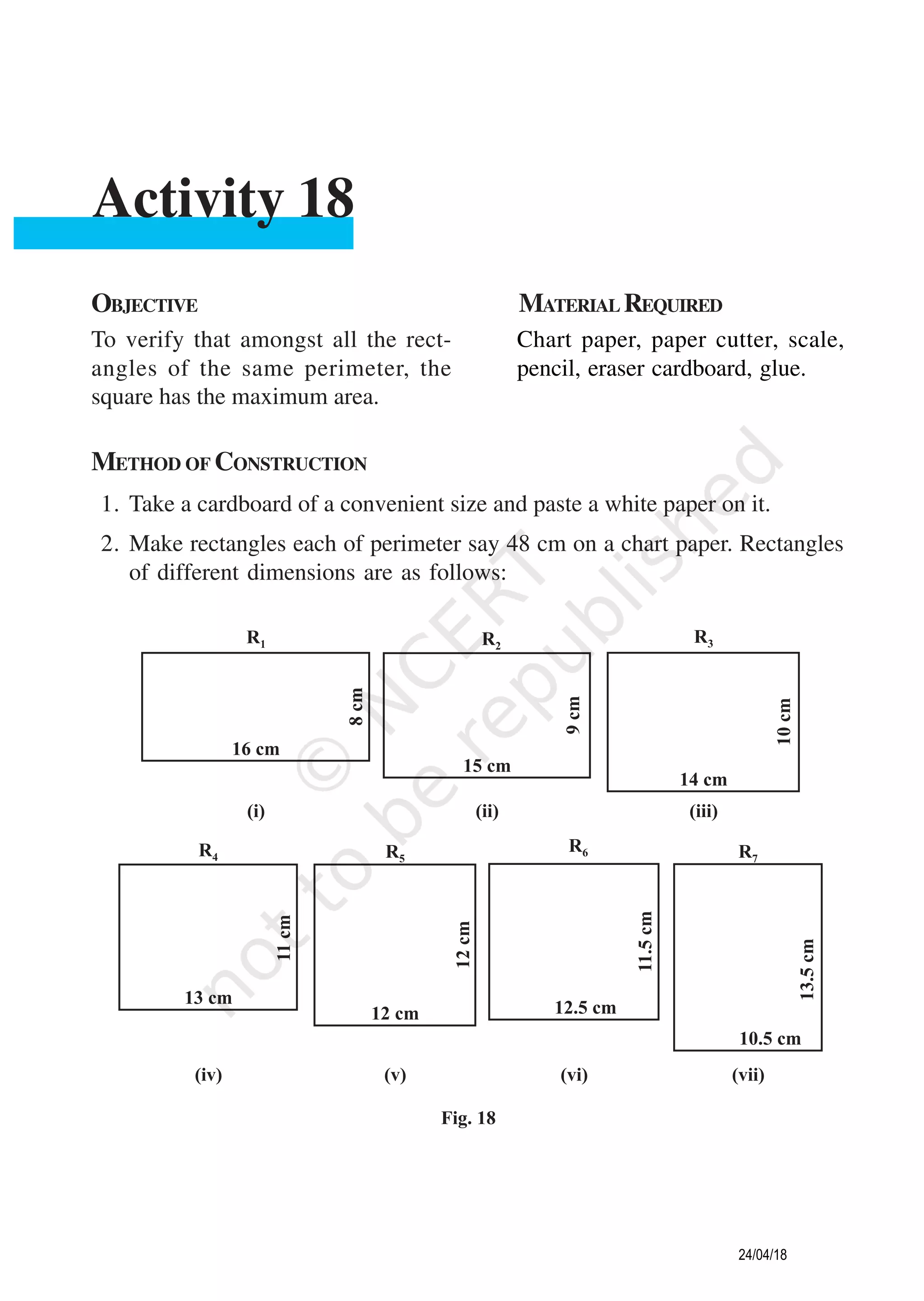
METHOD OF CONSTRUCTION
1. Fix a white chart paper of convenient size on a drawing board using adhesive.
2. Draw two perpendicular lines on the squared paper as the two rectangular axes.
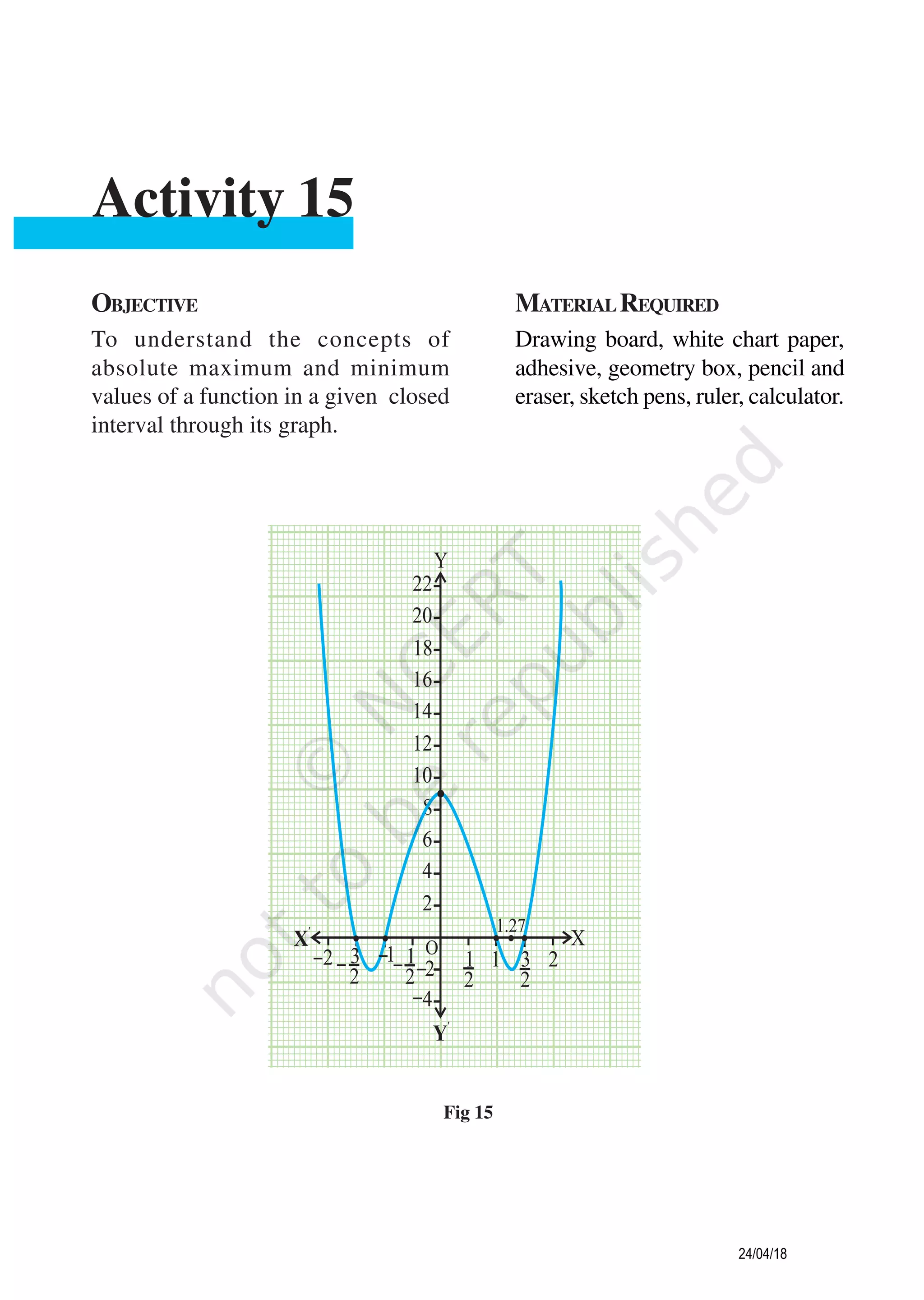
3. Graduate the two axes as shown in Fig.15.
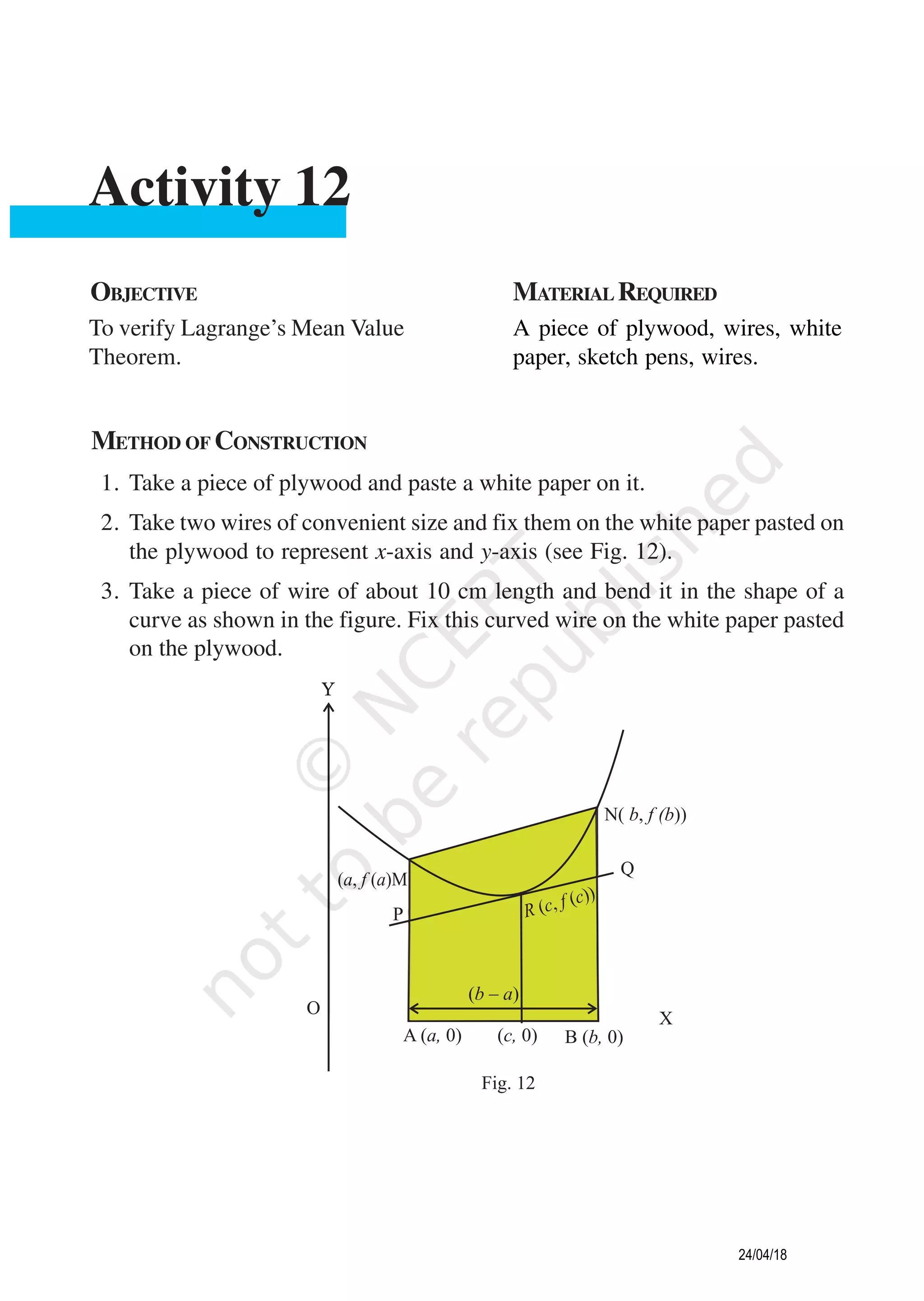
4. Let the given function be f (x) = (4x2
– 9) (x2
– 1) in the interval [–2, 2].
5. Taking different values of x in [–2, 2], find the values of f (x) and plot the
ordered pairs (x, f (x)).
6. Obtain the graph of the function by joining the plotted points by a free hand
curve as shown in the figure.
DEMONSTRATION
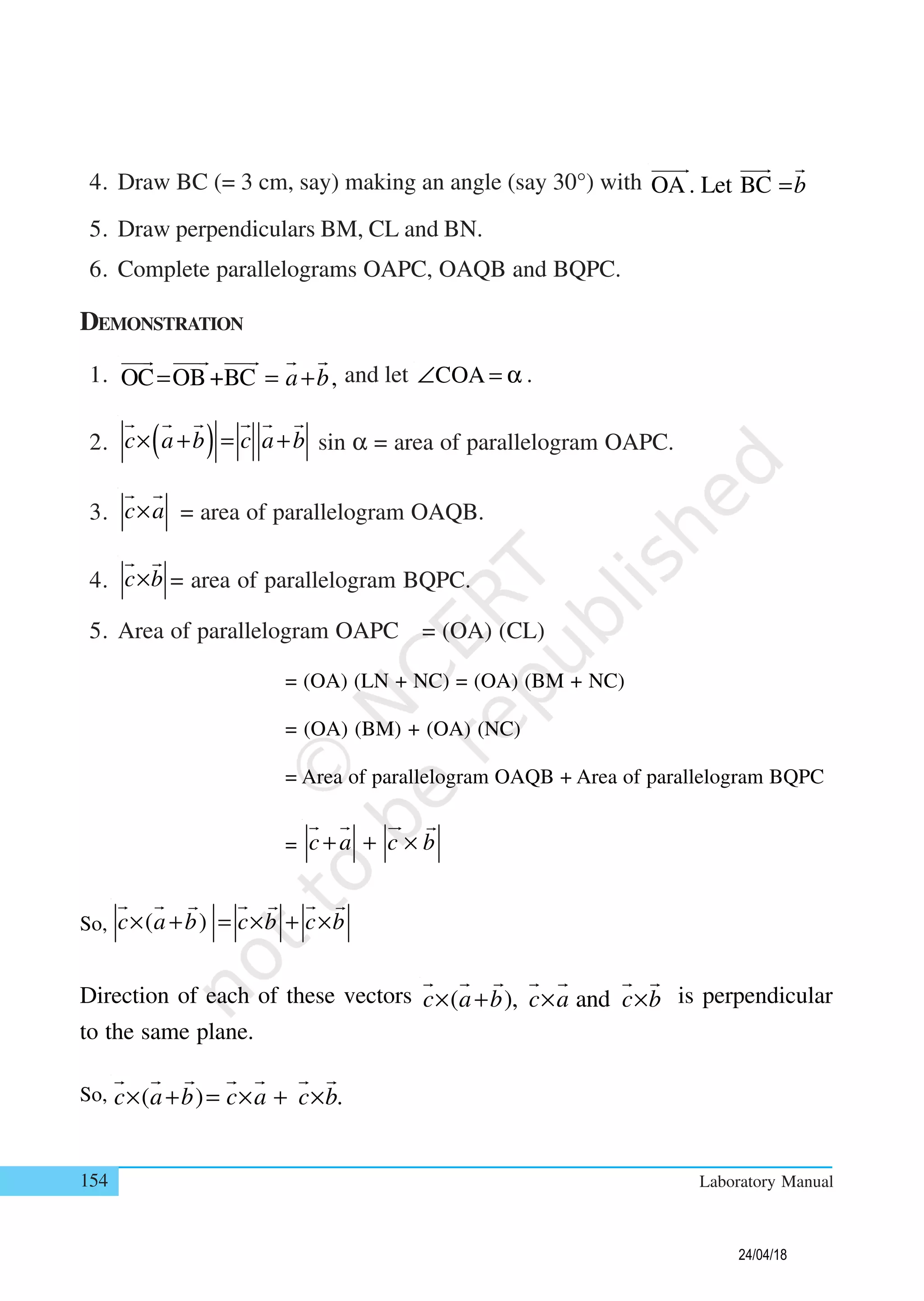
1. Some ordered pairs satisfying f (x) are as follows:
x 0 ± 0.5 ± 1.0 1.25 1.27 ± 1.5 ± 2
f (x) 9 6 0 – 1.55 –1.56 0 21
2. Plotting these points on the chart paper and joining the points by a free hand
curve, the curve obtained is shown in the figure.
OBSERVATION
1. The absolute maximum value of f (x) is ________ at x = ________.
2. Absolute minimum value of f (x) is ________ at x = _________.
APPLICATION
The activity is useful in explaining the concepts of absolute maximum / minimum
value of a function graphically.
24/04/18

13. Mathematics 139
NOTE
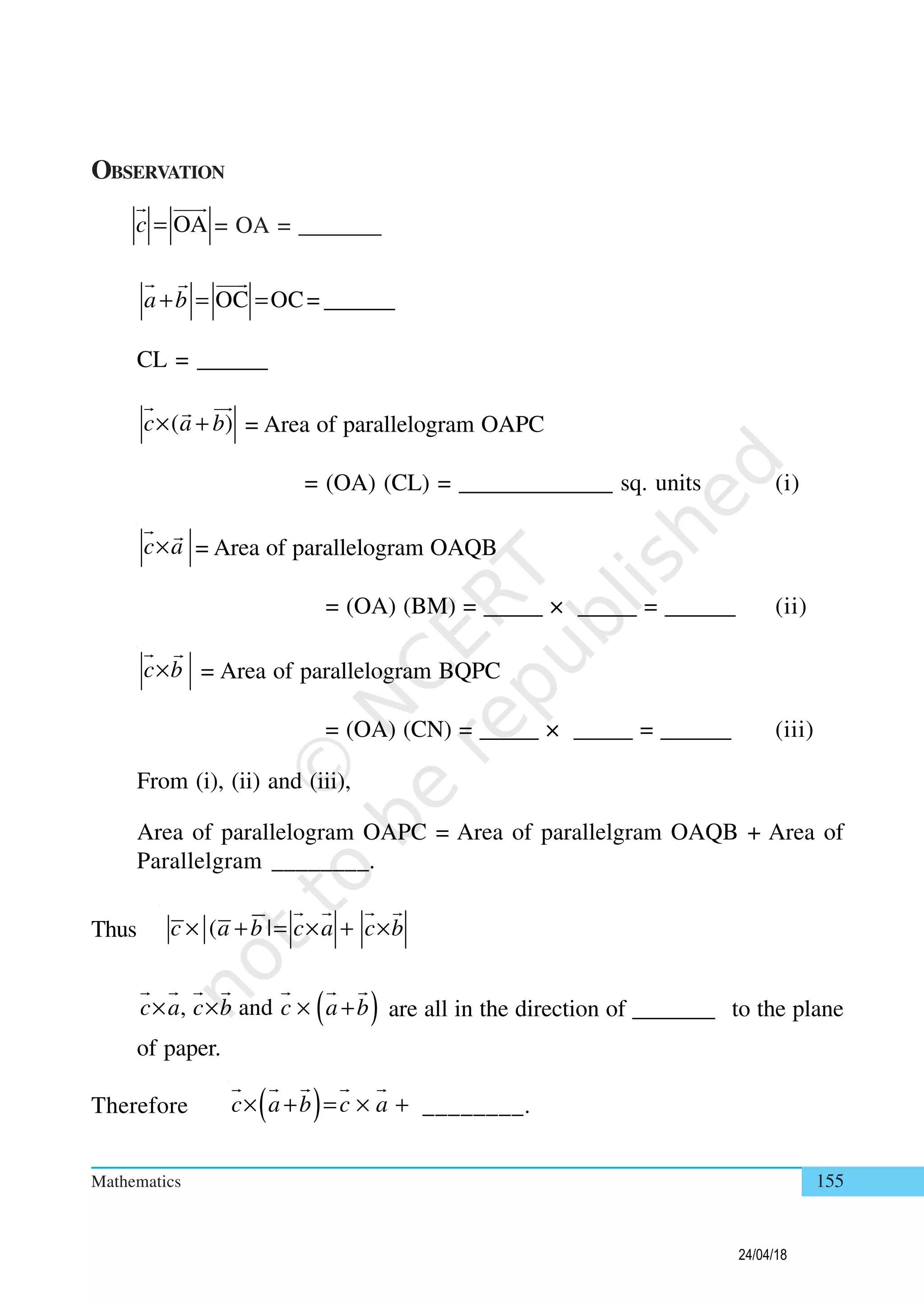
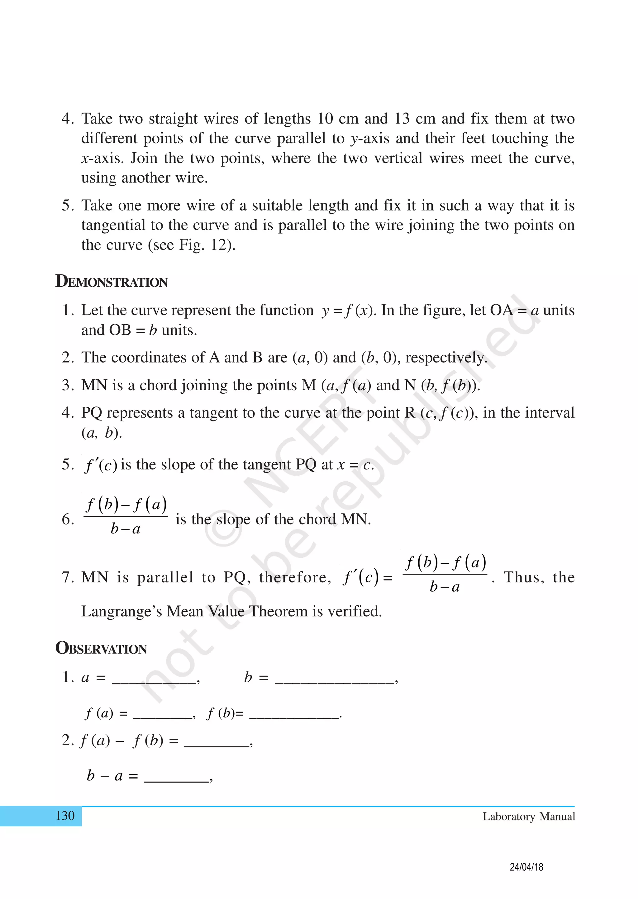
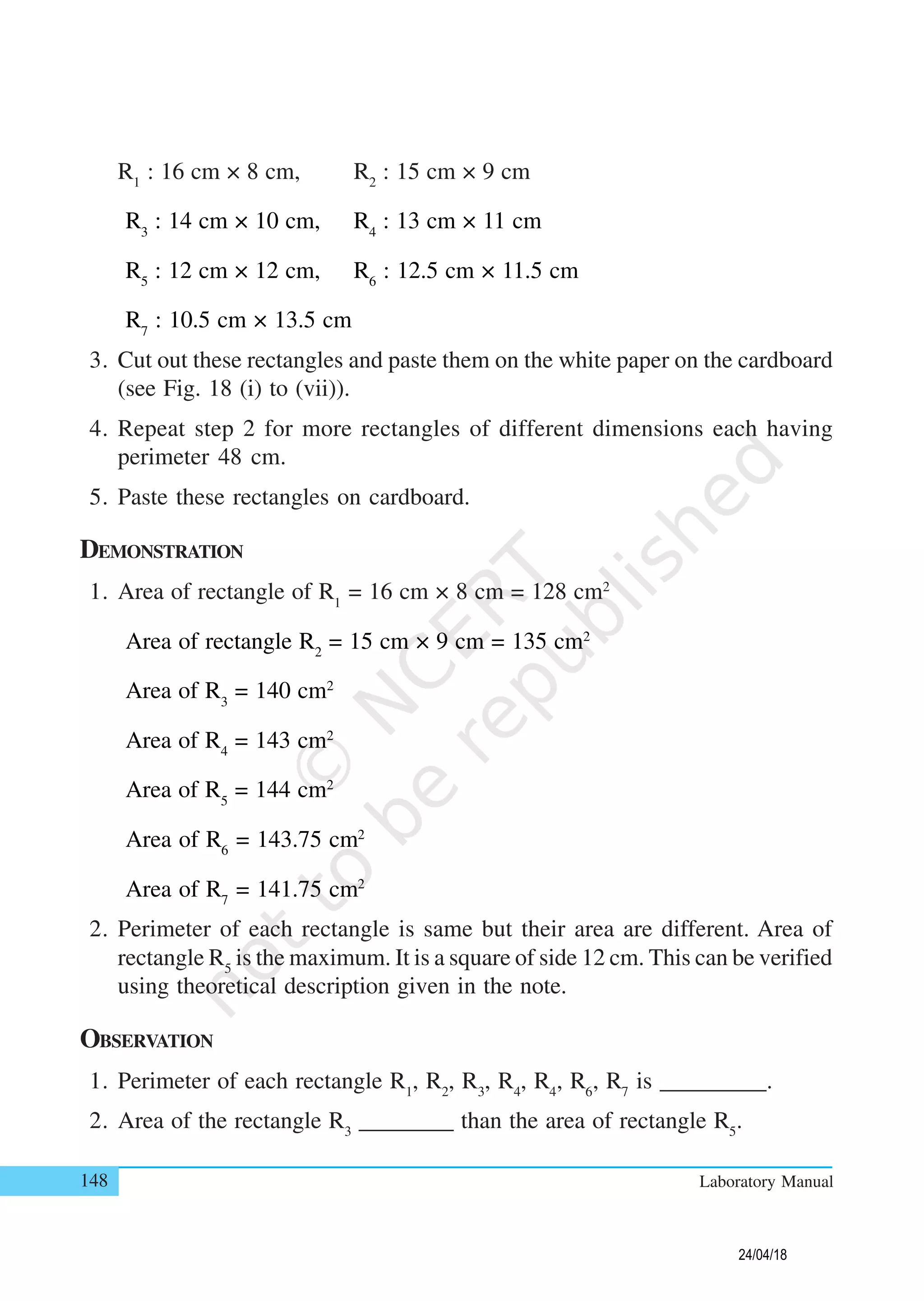
Consider f (x) = (4x2
– 9) (x2
– 1)
f (x) = 0 gives the values of x as
3
and 1
2
± ± . Both these values of x lie in the
given closed interval [–2, 2].
f ′ (x) = (4x2
– 9) 2x + 8x (x2
– 1) = 16x3
– 26x = 2x (8x2
– 13)
f ′ (x) = 0 gives
13
0, 1.27
8
x x= =± = ± . These two values of x lie in [–2, 2].
The function has local maxima/minima at x = 0 and x = ± 1.27, respectively.
24/04/18

14. METHOD OF CONSTRUCTION
1. Take a rectangular chart paper of size 20 cm × 10 cm and name it as ABCD.
2. Cut four equal squares each of side x cm from each corner A, B, C and D.
3. Repeat the process by taking the same size of chart papers and different
values of x.
4. Make an open box by folding its flaps using cellotape/adhesive.
OBJECTIVE MATERIAL REQUIRED
To construct an open box of maximum
volume from a given rectangular sheet
by cutting equal squares from each
corner.
Chart papers, scissors, cellotape,
calculator.
Activity 16
DEMONSTRATION
1. When x = 1, Volume of the box = 144 cm3
2. When x = 1.5, Volume of the box = 178.5 cm3
24/04/18

15. Mathematics 141
3. When x = 1.8, Volume of the box = 188.9 cm3
.
4. When x = 2, Volume of the box = 192 cm3
.
5. When x = 2.1, Volume of the box = 192.4 cm3
.
6. When x = 2.2, Volume of the box = 192.2 cm3
.
7. When x = 2.5, Volume of the box = 187.5 cm3
.
8. When x = 3, Volume of the box = 168 cm3
.
Clearly, volume of the box is maximum when x = 2.1.
OBSERVATION
1. V1
= Volume of the open box ( when x = 1.6) = .................
2. V2
= Volume of the open box ( when x = 1.9) = .................
3. V = Volume of the open box ( when x = 2.1) = .................
4. V3
= Volume of the open box ( when x = 2.2) = .................
5. V4
= Volume of the open box ( when x = 2.4) = .................
6. V5
= Volume of the open box ( when x = 3.2) = .................
7. Volume V1
is ____________ than volume V.
8. Volume V2
is ____________ than volume V.
9. Volume V3
is ____________ than volume V.
10. Volume V4
is ____________ than volume V.
11. Volume V5
is ____________ than volume V.
So, Volume of the open box is maximum when x = ________.
APPLICATION
This activity is useful in explaining the concepts of maxima/minima of functions.
It is also useful in making packages of maximum volume with minimum cost.
24/04/18

16. 142 Laboratory Manual
NOTE
Let V denote the volume of the box.
Now V = (20 – 2x) (10 – 2x) x
or V = 200x – 60x2
+ 4x3
2V
200–120 12
d
x x
dx
= + . For maxima or minima, we have,
V
0
d
dx
= , i.e., 3x2
– 30x + 50 = 0
i.e.,
30 900–600
7.9 or 2.1
6
x
±
= =
Reject x = 7.9.
2
2
V
–120 24
d
x
dx
= +
When x = 2.1,
2
2
Vd
dx
is negative.
Hence, V should be maximum at x = 2.1.
24/04/18

17. OBJECTIVE MATERIAL REQUIRED
To find the time when the area of a
rectangle of given dimensions become
maximum, if the length is decreasing
and the breadth is increasing at given
rates.
Chart paper, paper cutter, scale,
pencil, eraser, cardboard.
Activity 17
METHOD OF CONSTRUCTION
1. Take a rectangle R1
of dimensions 16 cm × 8 cm.
2. Let the length of the rectangle is decreasing at the rate of 1cm/second and
the breadth is increasing at the rate of 2 cm/second.
3. Cut other rectangle R2
, R3
, R4
, R5
, R6
, R7
, R8
, R9
, etc. of dimensions 15 cm ×
10 cm, 14 cm × 12 cm, 13 cm × 14 cm, 12 cm × 16 cm, 11 cm × 18 cm,
10 cm × 20 cm, 9 cm × 22 cm, 8 cm × 24 cm (see Fig.17).
4. Paste these rectangles on card board.
24/04/18

18. 144 Laboratory Manual
DEMONSTRATION
1. Length of the rectangle is decreasing at the rate of 1cm/s and the breadth is
increasing at the rate of 2cm/s.
2. (i) Area of the given rectangle R1
= 16 × 8 = 128 cm2
.
(ii) Area of rectangle R2
= 15 × 10 = 150 cm2
(after 1 sec).
(iii) Area of rectangle R3
= 168 cm2
(after 2 sec).
(iv) Area of rectangle R4
= 182 cm2
(after 3 sec).
(v) Area of rectangle R5
= 192 cm2
(after 4 sec).
(vi) Area of rectangle R6
= 198 cm2
(after 5 sec).
(vii) Area of rectangle R7
= 200 cm2
(after 6 sec).
(viii) Area of rectangle R8
= 198 cm2
(after 7 sec) and so on.
Thus the area of the rectangle is maximum after 6 sec.
OBSERVATION
1. Area of the rectangle R2
(after 1 sec) = __________.
2. Area of the rectangle R4
(after 3 sec) = __________.
3. Area of the rectangle R6
(after 5 sec) = __________.
4. Area of the rectangle R7
(after 6 sec) = __________.
5. Area of the rectangle R8
(after 7 sec) = __________.
6. Area of the rectangle R9
(after 8 sec) = __________.
7. Rectangle of Maximum area (after ..... seconds) = _______.
8. Area of the rectangle is maximum after _________ sec.
9. Maximum area of the rectangle is _________.
24/04/18

19. Mathematics 145
APPLICATION
This activity can be used in explaining the concept of rate of change and
optimisation of a function.
The function has local maxima/minima at x = 0 and x = ± 1.27, respectively.
Let the length and breadth of rectangle be a and b.
The length of rectangle after t seconds = a – t.
The breadth of rectangle after t seconds = b + 2t.
Area of the rectangle (after t sec) = A (t) = (a – t) (b + 2t) = ab – bt + 2at – 2t2
A′ (t) = – b + 2a – 4t
For maxima or minima, A′ (t) = 0.
NOTE
24/04/18

20. 146 Laboratory Manual
( )
2 –
A 0
4
a b
t t=′
( )A – 4t =′′
2 –
A – 4
4
a b
=′′ , which is negative
( )
2 –
Thus,A is maximumat
4
a b
t t = seconds.
Here, a = 16 cm, b = 8 cm.
Thus,
32 – 8 24
6
4 4
t = = = seconds
Hence, after 6 second, the area will become maximum.
24/04/18

21. METHOD OF CONSTRUCTION
1. Take a cardboard of a convenient size and paste a white paper on it.
2. Make rectangles each of perimeter say 48 cm on a chart paper. Rectangles
of different dimensions are as follows:
OBJECTIVE MATERIAL REQUIRED
To verify that amongst all the rect-
angles of the same perimeter, the
square has the maximum area.
Chart paper, paper cutter, scale,
pencil, eraser cardboard, glue.
Activity 18
24/04/18

22. 148 Laboratory Manual
R1
: 16 cm × 8 cm, R2
: 15 cm × 9 cm
R3
: 14 cm × 10 cm, R4
: 13 cm × 11 cm
R5
: 12 cm × 12 cm, R6
: 12.5 cm × 11.5 cm
R7
: 10.5 cm × 13.5 cm
3. Cut out these rectangles and paste them on the white paper on the cardboard
(see Fig. 18 (i) to (vii)).
4. Repeat step 2 for more rectangles of different dimensions each having
perimeter 48 cm.
5. Paste these rectangles on cardboard.
DEMONSTRATION
1. Area of rectangle of R1
= 16 cm × 8 cm = 128 cm2
Area of rectangle R2
= 15 cm × 9 cm = 135 cm2
Area of R3
= 140 cm2
Area of R4
= 143 cm2
Area of R5
= 144 cm2
Area of R6
= 143.75 cm2
Area of R7
= 141.75 cm2
2. Perimeter of each rectangle is same but their area are different. Area of
rectangle R5
is the maximum. It is a square of side 12 cm. This can be verified
using theoretical description given in the note.
OBSERVATION
1. Perimeter of each rectangle R1
, R2
, R3
, R4
, R4
, R6
, R7
is _________.
2. Area of the rectangle R3
________ than the area of rectangle R5
.
24/04/18

23. Mathematics 149
3. Area of the rectangle R6
_______ than the area of rectangle R5
.
4. The rectangle R5
has the diamensions ______ × ______ and hence it is a
________.
5. Of all the rectangles with same perimeter, the ________ has the maximum
area.
APPLICATION
This activity is useful in explaining the idea
of Maximum of a function. The result is also
useful in preparing economical packages.
Let the length and breadth of rectangle be x and y.
The perimeter of the rectangle P = 48 cm.
2 (x + y) = 48
or 24 or 24 –x y y x+ = =
Let A (x) be the area of rectangle, then
A (x) = xy
= x (24 – x)
= 24x – x2
A′ (x) = 24 – 2x
A′ (x) = ⇒ 24 – 2x = 0 ⇒ x = 12
A′′ (x) = – 2
A′′ (12) = – 2, which is negative
Therefore, area is maximum when x = 12
y = x = 24 – 12 = 12
So, x = y = 12
Hence, amongst all rectangles, the square has the maximum area.
NOTE
24/04/18

24. OBJECTIVE MATERIAL REQUIRED
To evaluate the definite integral
2
(1 )
b
a
x−∫ dx as the limit of a sum and
verify it by actual integration.
Cardboard, white paper, scale,
pencil, graph paper
Activity 19
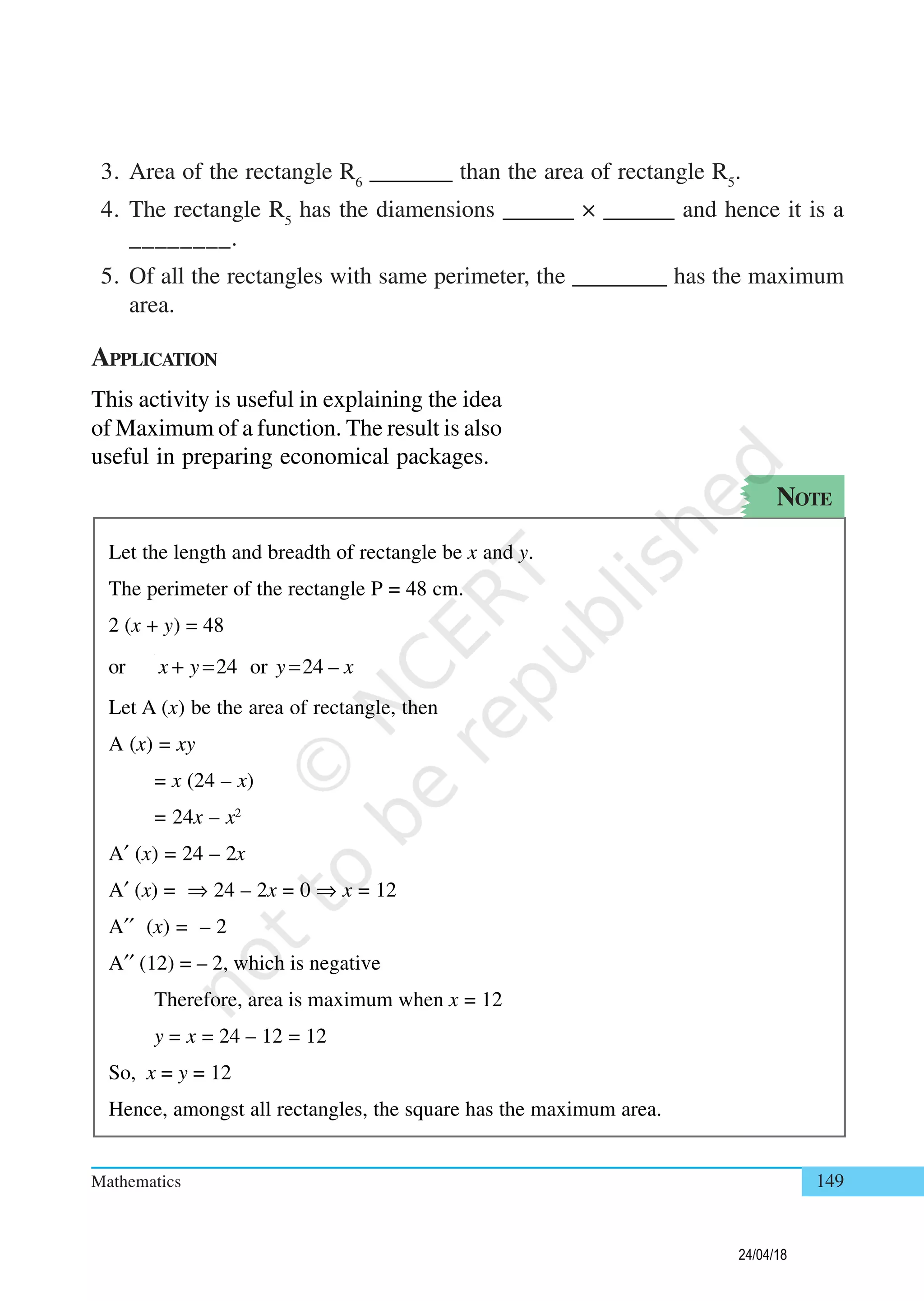
METHOD OF CONSTRUCTION
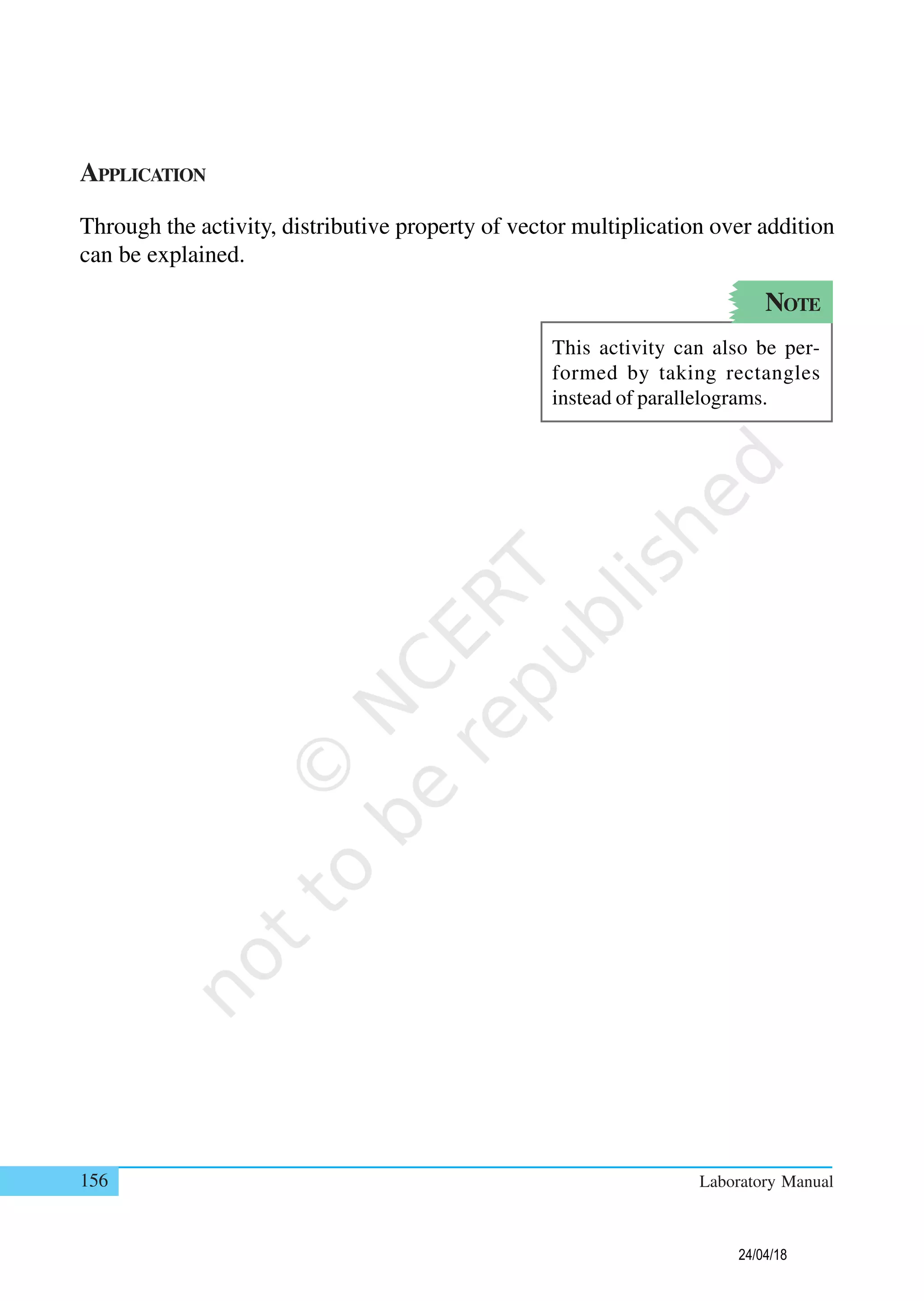
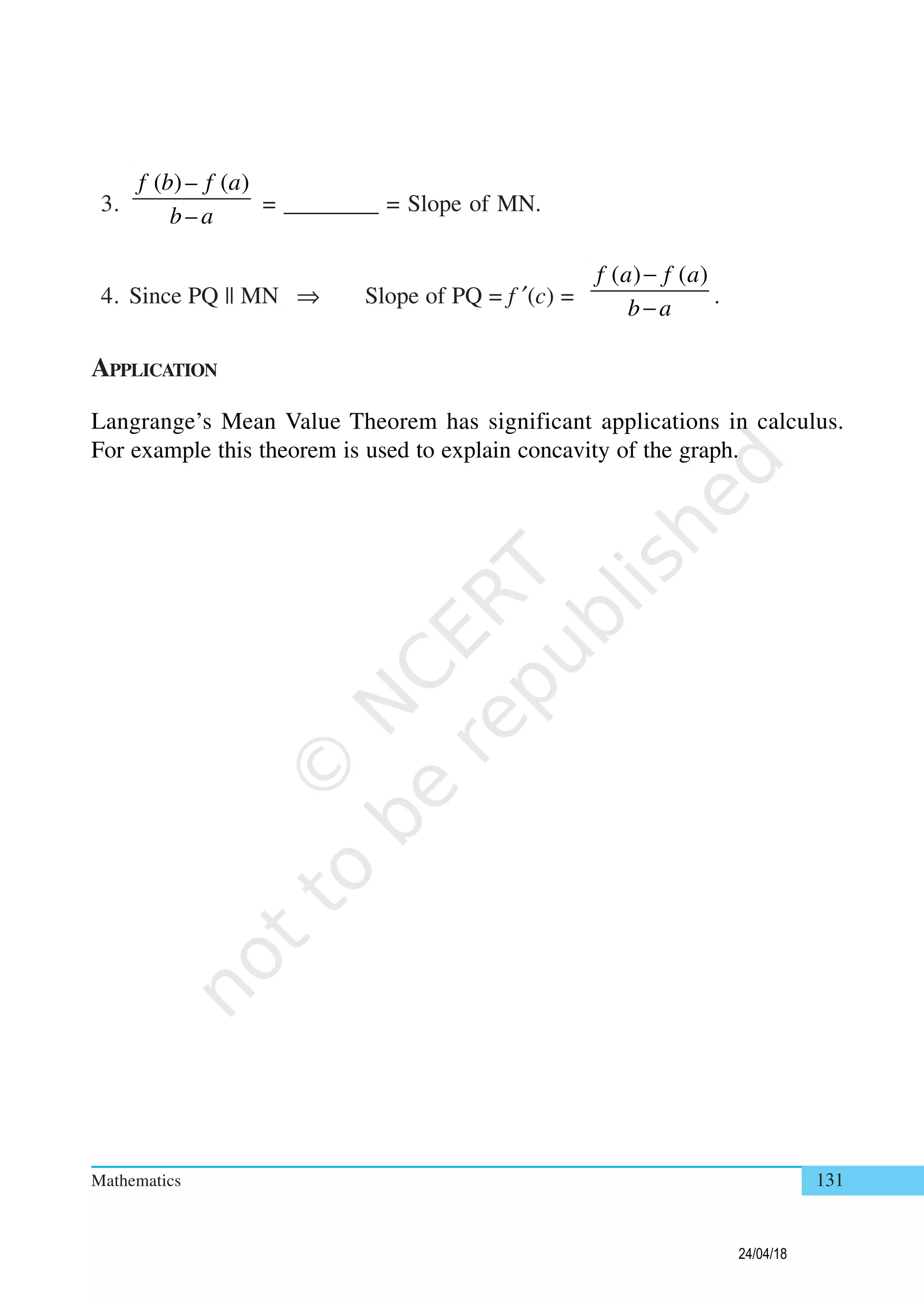
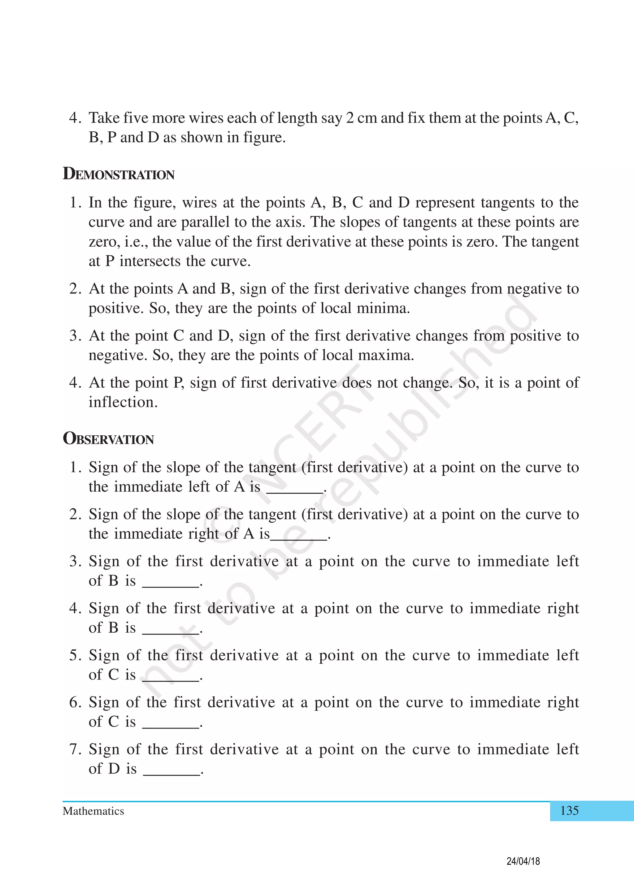
1. Take a cardboard of a convenient size and paste a white paper on it.
2. Draw two perpendicular lines to represent coordinate axes XOX′ and YOY′.
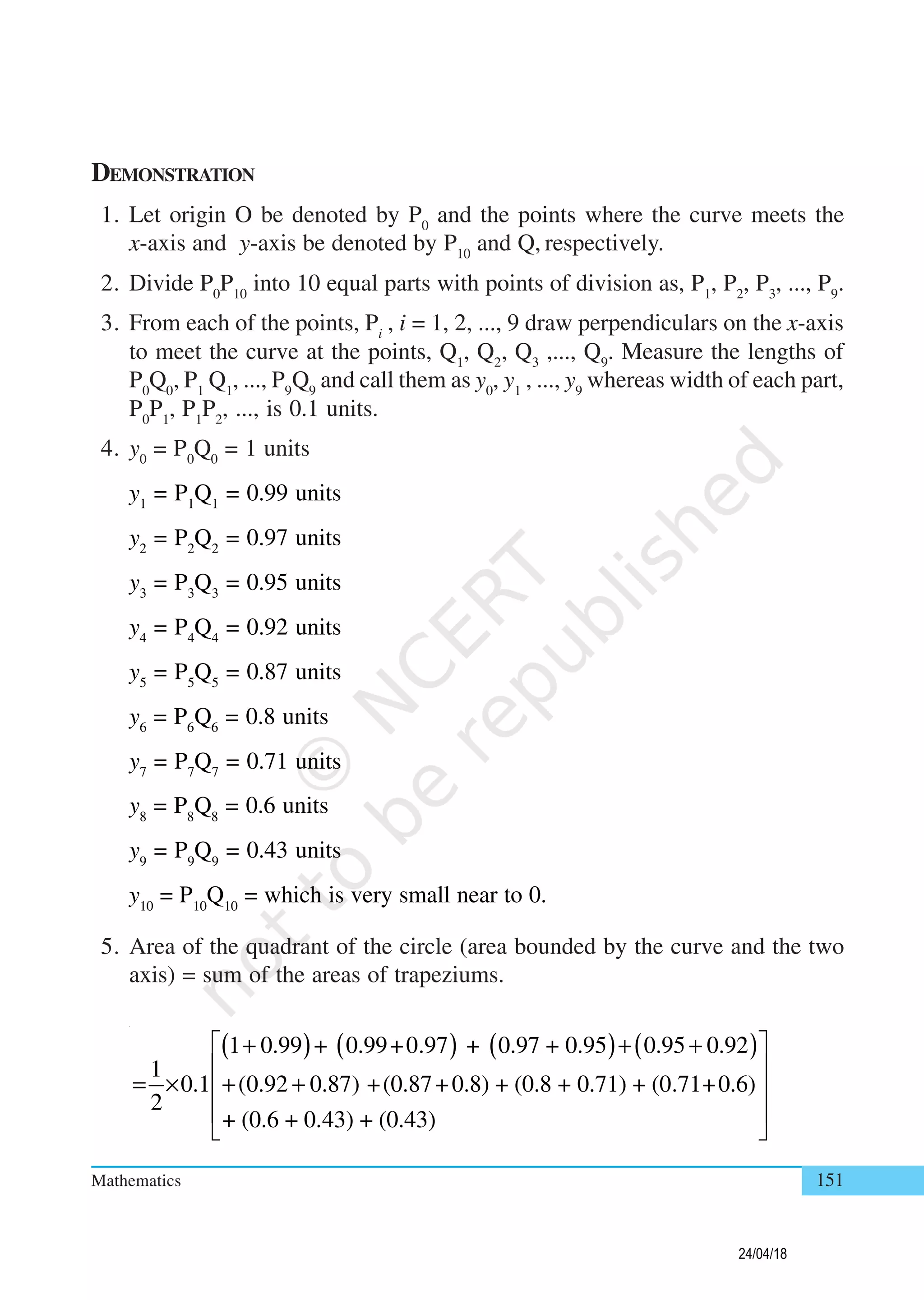
3. Draw a quadrant of a circle with O as centre and radius 1 unit (10 cm) as
shown in Fig.19.
The curve in the 1st quadrant represents the graph of the function 2
1 x− in the
interval [0, 1].
24/04/18

25. Mathematics 151
DEMONSTRATION
1. Let origin O be denoted by P0
and the points where the curve meets the
x-axis and y-axis be denoted by P10
and Q, respectively.
2. Divide P0
P10
into 10 equal parts with points of division as, P1
, P2
, P3
, ..., P9
.
3. From each of the points, Pi
, i = 1, 2, ..., 9 draw perpendiculars on the x-axis
to meet the curve at the points, Q1
, Q2
, Q3
,..., Q9
. Measure the lengths of
P0
Q0
, P1
Q1
, ..., P9
Q9
and call them as y0
, y1
, ..., y9
whereas width of each part,
P0
P1
, P1
P2
, ..., is 0.1 units.
4. y0
= P0
Q0
= 1 units
y1
= P1
Q1
= 0.99 units
y2
= P2
Q2
= 0.97 units
y3
= P3
Q3
= 0.95 units
y4
= P4
Q4
= 0.92 units
y5
= P5
Q5
= 0.87 units
y6
= P6
Q6
= 0.8 units
y7
= P7
Q7
= 0.71 units
y8
= P8
Q8
= 0.6 units
y9
= P9
Q9
= 0.43 units
y10
= P10
Q10
= which is very small near to 0.
5. Area of the quadrant of the circle (area bounded by the curve and the two
axis) = sum of the areas of trapeziums.
( ) ( ) ( ) ( )1 0.99 + 0.99+0.97 + 0.97 + 0.95 0.95 0.92
1
0.1 (0.92 0.87) +(0.87+0.8) + (0.8 + 0.71) + (0.71+0.6)
2
+ (0.6 + 0.43) + (0.43)
 + + +
 
= × + + 
 
 
24/04/18

26. 152 Laboratory Manual
= 0.1 [0.5 + 0.99 + 0.97 + 0.95 + 0.92 + 0.87 + 0.80 + 0.71 + 0.60 + 0.43]
= 0.1 × 7.74 = 0.774 sq. units.(approx.)
6. Definite integral =
1 2
0
1– x dx∫
1
2
1
0
1– 1 1 3.14
sin 0.785sq.units
2 2 2 2 4
x x
x−
  π
= + = × = = 
  
Thus, the area of the quadrant as a limit of a sum is nearly the same as area
obtained by actual integration.
OBSERVATION
1. Function representing the arc of the quadrant of the circle is y = ______.
2. Area of the quadrant of a circle with radius 1 unit =
1
2
0
1– x∫ dx = ________.
sq. units
3. Area of the quadrant as a limit of a sum = _______ sq. units.
4. The two areas are nearly _________.
APPLICATION
This activity can be used to demonstrate the
concept of area bounded by a curve. This
activity can also be applied to find the
approximate value of π.
NOTE
Demonstrate the same activity
by drawing the circle x2
+ y2
= 9
and find the area between x = 1
and x = 2.
24/04/18

27. METHOD OF CONSTRUCTION
1. Fix a white paper on the cardboard.
2. Draw a line segment OA (= 6 cm, say) and let it represent c .
3. Draw another line segment OB (= 4 cm, say) at an angle (say 60°) with OA.
Let OB a=
OBJECTIVE MATERIAL REQUIRED
To verify geometrically that
( )c a b c a c b× + = × + ×
Geometry box, cardboard, white
paper, cutter, sketch pen, cellotape.
Activity 20
24/04/18

28. 154 Laboratory Manual
4. Draw BC (= 3 cm, say) making an angle (say 30°) with OA . Let BC b=
5. Draw perpendiculars BM, CL and BN.
6. Complete parallelograms OAPC, OAQB and BQPC.
DEMONSTRATION
1. OC OB +BC ,a b= = + and let COA∠ = α .
2. ( )c a b c a b× + = + sin α = area of parallelogram OAPC.
3. c a× = area of parallelogram OAQB.
4. c b× = area of parallelogram BQPC.
5. Area of parallelogram OAPC = (OA) (CL)
= (OA) (LN + NC) = (OA) (BM + NC)
= (OA) (BM) + (OA) (NC)
= Area of parallelogram OAQB + Area of parallelogram BQPC
= c a c b+ + ×
So, ( )c a b c b c b× + = × + ×
Direction of each of these vectors ( ), andc a b c a c b× + × × is perpendicular
to the same plane.
So, ( ) .c a b c a c b× + = × + ×
24/04/18

29. Mathematics 155
OBSERVATION
OAc = = OA = _______
OC OC= ______a b+ = =
CL = ______
( )c a b× + = Area of parallelogram OAPC
= (OA) (CL) = _____________ sq. units (i)
c a× = Area of parallelogram OAQB
= (OA) (BM) = _____ × _____ = ______ (ii)
c b× = Area of parallelogram BQPC
= (OA) (CN) = _____ × _____ = ______ (iii)
From (i), (ii) and (iii),
Area of parallelogram OAPC = Area of parallelgram OAQB + Area of
Parallelgram ________.
Thus ( |c a b c a c b× + = × + ×
( ), andc a c b c a b× × × + are all in the direction of _______ to the plane
of paper.
Therefore ( )c a b c a× + = × + ________.
24/04/18

30. 156 Laboratory Manual
APPLICATION
Through the activity, distributive property of vector multiplication over addition
can be explained.
NOTE
This activity can also be per-
formed by taking rectangles
instead of parallelograms.
24/04/18