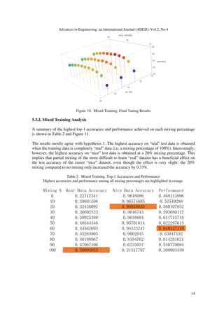
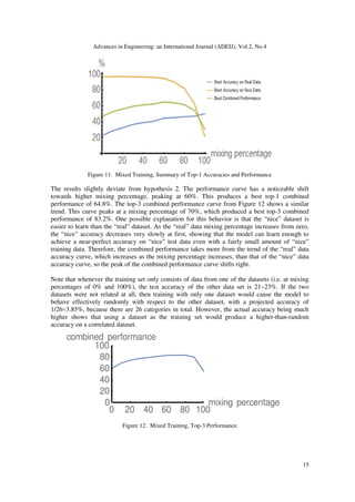
This research investigates a convolutional neural network training method using two datasets with differing characteristics, achieving enhanced performance through mixed training. The study found that combining datasets at a 70% ratio significantly improved classification accuracy, with a top-1 performance of 63.8% compared to 30.8% without mixing. Additionally, the research highlights that iterative training significantly underperforms mixed training due to fast forgetting issues.
![Advances in Engineering: an International Journal (ADEIJ), Vol.2, No.4
1
A STUDY OF METHODS FOR TRAINING WITH
DIFFERENT DATASETS IN IMAGE CLASSIFICATION
Yuxuan Bao
Northfield Mount Hermon School
ABSTRACT
This research developed a training method of Convolutional Neural Network model with multiple datasets
to achieve good performance on both datasets. Two different methods of training with two
characteristically different datasets with identical categories, one with very clean images and one with
real-world data, were proposed and studied. The model used for the study was a neural network derived
from ResNet. Mixed training was shown to produce the best accuracies for each dataset when the dataset is
mixed into the training set at the highest proportion, and the best combined performance when the real-
world dataset was mixed in at a ratio of around 70%. This ratio produced a top-1 combined performance
of 63.8% (no mixing produced 30.8%) and a top-3 combined performance of 83.0% (no mixing produced
55.3%). This research also showed that iterative training has a worse combined performance than mixed
training due to the issue of fast forgetting.
KEYWORDS
Supervised Learning, Image Classification, Convolutional Neural Network, ResNet, Multiple Datasets
1. INTRODUCTION
Image classification through machine learning can be applied to many different problems, such as
product defect checking in factories, product sorting in warehouses, and object identification for
everyday use. Currently, many large datasets (for example, ImageNet) are available for use to aid
in the training of models to perform image classification. However, there is often great difficulty
in using multiple available datasets for the desired categories for a given application, because the
different datasets usually have different characteristics that may or may not correspond with the
desired application. This research examines the effects of training a convolutional neural network
model using two datasets with drastically different characteristics but contain the same categories,
using different methods of training and ratios of mixing the datasets, with the goal of developing
a method of training with multiple datasets that has good performance on both datasets.
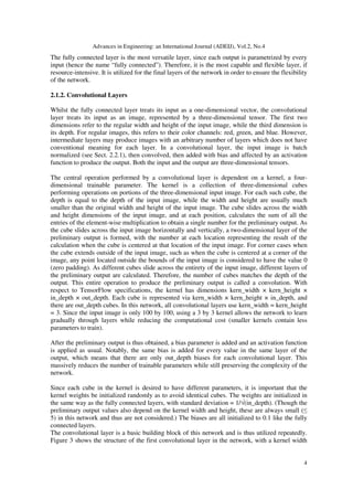
2. NETWORK STRUCTURE
The structure of the neural network model used for this study is a deep neural network with 25
layers, based on the design of the 34-layer ResNet proposed in [1]. The structure is shown in
Table 1, while a graphic representation of the network is shown in Figure 1. The details of each of
the layers, operations, and blocks, including modifications to the original and rationale for those
modifications, are discussed in this section.
2.1. Layers
Layers are the basic building blocks of the neural network model. The model used is very deep
and contains many of these layers.](https://image.slidesharecdn.com/2419adeij011-190705090728/85/A-STUDY-OF-METHODS-FOR-TRAINING-WITH-DIFFERENT-DATASETS-IN-IMAGE-CLASSIFICATION-1-320.jpg)
![Advances in Engineering: an International Journal (ADEIJ), Vol.2, No.4
7
the residual blocks and an average pooling layer after the last convolutional layer in order to
reduce the computational cost of the succeeding fully connected layer.
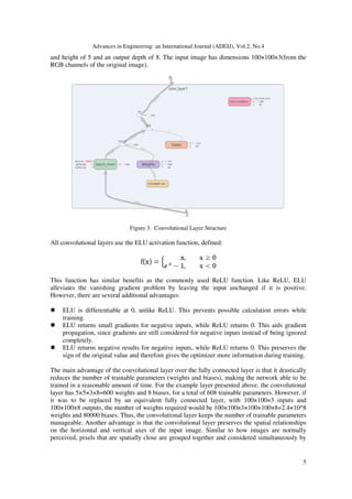
2.3. RESIDUAL BLOCKS
Residual blocks are made up of two convolutional layers and a bridge that transfers the input of
the first layer to the output of the second layer, adding them together to produce the output of the
entire block. The activation function of the second convolutional layer is applied after the original
input is added. The central idea is that the network may learn to either use the two layers or to
omit them (by learning to push the weights of the two layers to 0). Thus, if the network
encounters problems trying to optimize a large network, it may be able to shrink the network and
optimize the smaller network instead. For a more detailed discussion of the benefits of residual
blocks, see [1].
2.3.1. Same-size Residual Block
The residual block is easier to build when the input of the first convolutional layer has the exact
same dimensions as the output of the second convolutional layer, that is, the two convolutional
layers do not modify the size of the image. When this is the case, the first input can simply be
element-wise added to the second output. Figure 4 shows a same-size residual block with the
dimensions of all images at 50×50×8.
2.3.2. Changing-size Residual Block
Building a residual block is trickier when the convolutional layer changes the dimensions of the
input image. Since the dimensions of the first input does not match that of the second output, they
cannot be directly added together. Instead, a special convolutional layer is added to transform the
first input to the proper dimensions. This special convolutional layer uses a kernel with
dimensions 1 × 1 × in_depth × out_depth, and uses a stride equal to the stride of the convolutional
layer that changed the image’s dimensions. This will allow the output for this special
convolutional layer to match the second output exactly in dimensions, while mostly preserving
the values of the input image. The 1×1 convolutions will produce different linear combinations of
the input layers for each output layer, and the stride size will omit data in between the strides to
reduce image size. After this layer, the results can be element-wise added to the second output as
usual. Figure 5 shows a changing-size residual block with input dimensions 50×50×8 and output
dimensions 25×25×16.
3. TRAINING
This section describes the details of how the model is trained. This research uses the Tensorflow
framework [3] in Python to train and test the neural network models.](https://image.slidesharecdn.com/2419adeij011-190705090728/85/A-STUDY-OF-METHODS-FOR-TRAINING-WITH-DIFFERENT-DATASETS-IN-IMAGE-CLASSIFICATION-7-320.jpg)
![Advances in Engineering: an International Journal (ADEIJ), Vol.2, No.4
10
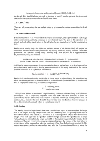
4.1. DATASET 1 (NICE DATASET)
The first dataset is taken from part of the Fruits-360 dataset, a free online database of fruits from
[2]. This dataset consists of very nice fruit images. Every image is exactly 100 by 100 pixels
wide, has a completely white background, and always contains only one fruit in each image. A
typical image from Dataset 1 is shown in Figure 6.
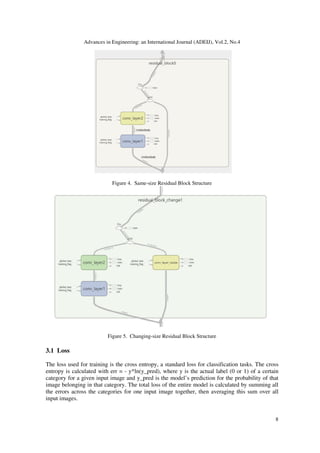
4.2. DATASET 2 (REAL DATASET)
The second dataset is personally gathered as part of the research, and comes from web image
searches of the 26 fruit types. In contrast to Dataset 1, this dataset mostly contains rectangular
images with non-white backgrounds and may contain multiple fruits in the same picture. Each of
these images are cropped into square images (cutting out the edges that are longer, horizontal or
vertical), then resized down to 100x100 pixels as part of the program before being fed into the
models. However, to keep some things consistent with Dataset 1, all images from Dataset 2 show
only the exteriors of each fruit, and will never show a cut-open fruit. A typical image from
Dataset 2 is shown in Figure 7.
Figure 6. Nice Data Example
Figure 7. Real Data Example
4.3. TEST SETS
One test set is created from each dataset by randomly taking 40% of the images in each category
out. This process forms Test Set 1 (Nice Test Set) and Test Set 2(Real Test Set). The performance
of models on these datasets is used to evaluate the general accuracy of the models. Whenever a
model is tested, it is run on both test sets to give accuracies for each test set, so its performance
could be measured for both datasets.
4.4. TRAINING SETS AND TRAINING METHODS
The other 60% of the images from the two datasets form the “nice” and “real” training sets.
Images from these training sets are used to train the models. Based on the training method,
different sets of images are used from these training sets. The two training methods described in
the following subsections are used because they have the advantage of low computational cost.
Both methods only require a single model to be trained, and require no additional processing
beyond partitioning the dataset randomly. The experiment thus studies the performance of these
training methods which only require minimal computational power beyond the base cost of
training one model itself.](https://image.slidesharecdn.com/2419adeij011-190705090728/85/A-STUDY-OF-METHODS-FOR-TRAINING-WITH-DIFFERENT-DATASETS-IN-IMAGE-CLASSIFICATION-10-320.jpg)

![Advances in Engineering: an International Journal (ADEIJ), Vol.2, No.4
18
exhibit similar behavior. Similarly, the study is constrained to image classification tasks and
differences may be observed for other tasks.
The images used as dataset in this study are relatively small in size (all images are
normalized to 100x100 px). This also implies a thin network, with few trainable parameters
every layer compared to CNNs used in most other studies. A larger network may produce
different results.
Both training methods studied use only one trained CNN to perform the classification task.
Methods that use more than one model may perform better in accuracy, but would be more
computationally expensive.
8. CONCLUSION
Two different methods of training with two characteristically different datasets with identical
categories were proposed and studied. The model used for the study was a neural network derived
from ResNet. The correlation between the two datasets caused a higher-than-random accuracy on
one dataset when only data from the other dataset was used to train the model. Mixed training
was shown to produce the best accuracies for each dataset when the dataset is mixed into the
training set at the highest proportion, and the best combined performance when slightly more of
the more difficult to learn dataset was mixed in than the other dataset. Iterative training was
shown to have a worse combined performance than mixed training due to the issue of fast
forgetting, and also performs worse than mixed training in terms of accuracies of individual
datasets.
ACKNOWLEDGEMENTS
The author would like to thank the Chinese Academy of Sciences for providing computational
power for this research.
REFERENCES
[1] He, K., Zhang, X., Ren, S., & Sun, J. (2015, December 10). Deep residual learning for image
recognition. Retrieved from Arxiv database. (Accession No. arXiv:1512.03385v1)
[2] Muresan, H., & Oltean, M. (2018). Fruit recognition from images using deep learning. Acta
Universitatis Sapientiae, Informatica, 10(1), 26-42. Abadi, M., Agarwhal, A., Barham,P., Brevdo, E.,
Chen, Z., Citro, C., . . . Zheng, X. (2016, March 16).
[3] TensorFlow: Large-Scale machine learning on heterogeneous distributed systems. Retrieved from
Arxiv database. (Accession No. arXiv:1603.04467v2)
AUTHOR
Yuxuan BaoYuxuan is a high school senior at Northfield Mount Hermon School in Gill,
MA. He enjoys compu ter science very much and is excited about the capabilities of
artificial intelligence. He is in the platinum division of the USACO contest.](https://image.slidesharecdn.com/2419adeij011-190705090728/85/A-STUDY-OF-METHODS-FOR-TRAINING-WITH-DIFFERENT-DATASETS-IN-IMAGE-CLASSIFICATION-18-320.jpg)