1. Proceeding of the 6th
International Symposium on Artificial Intelligence and Robotics & Automation in Space:
i-SAIRAS 2001, Canadian Space Agency, St-Hubert, Quebec, Canada, June 18-22, 2001.
Continuous Measurements and Quantitative Constraints - Challenge Problems for
Discrete Modeling Techniques
Charles H. Goodrich, Dynacs Engineering,
Kennedy Space Center, FL
Charles.Goodrich@ksc.nasa.gov
James Kurien
NASA Ames Research Center
jkurien@arc.nasa.gov
Keywords model-based diagnosis, discrete models,
constraints, modeling, in-situ resource utilization.
Abstract
Many techniques in artificial intelligence operate on
discrete models, wherein each variable of a system
description may take on only a finite number of
discrete values. These discrete models are easy to
acquire, they have computational advantages, and
there are many well-developed algorithms for
manipulating them. In contrast, the world presents us
with many continuous processes we would like to
simulate, identify or control. Many discrete techniques
from AI are regularly applied to discrete abstractions
of continuous processes. This of course is not always
possible. It’s therefore important to consider whether
one’s continuous problem lends itself to being
abstracted and solved as a discrete problem. We
describe a set of modeling technique and algorithms
for discrete, model-based diagnosis and control, in a
manner we hope will be accessible to those outside the
field. We then present a continuous problem in the
domain of spacecraft state identification and control
for which a discrete abstraction of the problem allows
us to perform useful diagnosis and reconfiguration.
We then present a seemingly similar problem for
which developing a discrete abstraction was quite
difficult and which did not result in as useful a
diagnosis and control system. We contrast the two
systems, and describe some of the problems that made
the second problem far less suitable for use with a
discrete model and discrete reasoning algorithms.
1 Introduction
Suppose we would like to create algorithms that
perform computations about a physical system such as
a spacecraft in order to perform tasks such as
diagnosing its current condition, simulating its future
operation, or planning a set of control inputs to move
the system to a desired condition. In order to use
such algorithms, we will require a model or formal
description of the physical system. A continuous
model includes real-valued attributes that may take on
an infinite number of values and continuous functions
that compute the value of one attribute from another.
Change is modeled as the derivative of one or more
attributes over time. For example, a model of heating
and cooling of a spacecraft might include continuous
variables that represent the energy radiated from the
spacecraft into space and the energy output of its
heaters, and a set of differential equations that model
thermal conductivity through the spacecraft’s
structure. When we begin to model complete systems,
we may often find that the physical behavior of the
system is continuous, but that a controller with
discrete states controls it. A hybrid model includes
both discrete states and continuous variables. A
hybrid model can discretely transition from one state
to another, and within each state can evolve
continuously through a set of differential equations.
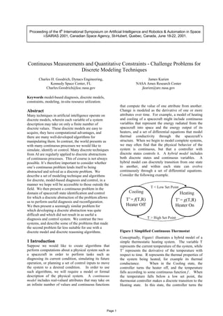
Consider the following example.
T < Low Set Point
Cooling
T’= f(T,R)
Heater Off
T > High Set Point
Heating
T’= g(T,R)
Heater On
Figure 1 Simplified Continuous Thermostat
Conceptually, Figure1 illustrates a hybrid model of a
simple thermostatic heating system. The variable T
represents the current temperature of the system, while
T’ represents the derivative of the temperature with
respect to time. R represents the thermal properties of
the system being heated, for example its thermal
conductance. When in the Cooling state, the
controller turns the heater off, and the temperature
falls according to some continuous function f . When
the temperature falls below a low set point, the
thermostat controller makes a discrete transition to the
Heating state. In this state, the controller turns the
Page 1

2. heater on, and the temperature rises according to some
continuous function g. Such a model would help us to
simulate the temperature of the system given the set
points and the parameter R, would be useful in
diagnosing whether the heater was operating properly,
and so on.
While much of the world is hybrid, a significant
amount of work in artificial intelligence concerns
discrete models. In contrast to a continuous model,
each attribute of a discrete model may take on only a
finite number of discrete values. Thus, there is only a
finite (though possibly very large) set of states the
discrete model can attain. Using a discrete model has
computational advantages, and a wide range of
discrete modeling formalisms and algorithms have
been developed or applied by the AI community.
Examples of techniques that apply to discrete models
include STRIPS-style planning and many of its
extensions (see Boutilier, Dean & Hanks, 1995 for an
overview), partially observable Markov decision
processes (see Kaelbling, Littman & Cassandra), some
of the work in model-based diagnosis (see Hamscher,
Console & deKleer 1992 for an overview), and
anything that makes use of a propositional logic
encoding.
Fortunately, we can often capture the features of our
hybrid system that are relevant to a particular task
(e.g., planning, diagnosis, simulation or so on) in a
discrete abstraction. That is, we can abstract an
infinite number of hybrid behaviors into a finite
number of discrete behaviors. For example, to
determine whether or not the thermostat of Figure 1 is
functioning correctly, it may be sufficient to create the
discrete model illustrated in Figure 2. When the
temperature level drops below a set point, the system
enters the discrete heating state, wherein the heater
must be on and the temperature must be rising. Any
continuous behavior that fits this discrete description
is normal behavior, and any that does not indicates a
failure.
T < Low Set Point
Cooling
T’< 0
Heater Off
T >High Set Point
Heating
T’>= 0
Heater On
Figure 2 Qualitative Thermostat Model
If a discrete abstraction such as this provides sufficient
information for the task at hand, then we may then
apply our discrete techniques. Discrete abstractions
are regularly applied in AI with great success.
Examples of their use are too numerous to enumerate,
but they include robot navigation (for example,
Nourbakhsh, Powers & Birchfield, 1996), and
spacecraft diagnosis and control (for example,
Williams & Nayak, 1996).
The issue is then, when is a discrete abstraction
sufficient, when is it insufficient, and how does one
determine this before investing time writing a discrete
model. We have spent the last few years applying
discrete diagnosis and control systems to a variety of
domains (Bernard, et al, 1998; Kurien, Nayak &
Williams, 1998). In the following sections of the
paper, we first describe a typical application to which
we have applied discrete diagnosis and control
techniques. We then give an intuition of how one
particular discrete diagnosis and control system, called
Livingstone (Williams & Nayak, 1996; Kurien &
Nayak, 2000) operates and provide some intuitions on
why it works well on the typical application. We then
describe a domain that appears to be similar where
discrete abstractions worked rather poorly. We then
describe the types of problems that separate the two
domains, and what capabilities a hybrid diagnosis and
control system needs to have to address the more
complex domain.
3 The Propulsion System Application
Figure 3 illustrates the redundant propulsion system
used in the Cassini spacecraft, designed to last a seven
year cruise to Saturn and autonomously insert itself
into orbit around Saturn. The purpose of the system is
to provide the appropriate amount of acceleration by
combining fuel and an oxidizer in an engine for a
specified amount of time. The helium tank is filled
with helium under high pressure. Conceptually,
controlling the system is straightforward. When the
appropriate valves are opened, the high pressure in the
helium tank pressurizes the oxidizer and fuel tanks.
This forces oxygen and fuel into the engine where it is
ignited to produce thrust. When sufficient thrust is
achieved, the valves are closed.
Page 2

3. Helium tank
Fuel tank
Oxidizer Tank
Main
Engines
Valve
Pyro valve
Pyro ladder
Regulator
Figure 3- Engine Schematic
In actuality, the control problem is complicated by the
redundancy needed to ensure success on a long
mission. Two engines are provided in the case that one
fails. Each engine is supplied with fuel and oxidizer
through a complex arrangement of valves. Valves or
pipe branches in parallel ensure that if valves stick
closed, a redundant parallel valve can be used to allow
fluid flow. Valves in series ensure that if valves stick
open, an upstream valve can be closed to prevent fluid
flow. Not shown are valve drivers that control the
latch valves and a set of flow, pressure and
acceleration sensors that provide partial observability
of the system. There are approximately 1015
possible
configurations of the system including failures.
Several hundred of those configurations produce
thrust, depending upon which valves are open or
closed. Given a set of failures, thrust configurations
that can be reached without using a pyro valve are
preferred, as pyro valves can only be opened or closed
once. Regardless of the number of failures that occur,
we’d like the control system to determine the current
configuration of the propulsion system and find the
best viable configuration of the system that will
produce thrust.
Though this system is relatively complex, using only a
discrete model we can answer the question of which
valves are stuck open or closed and what actions
should be taken to create a route for fuel and oxidizer
to a working engine. The next section describes how
this is accomplished.
2 Discrete Diagnosis & Control
Our discrete model of a hardware system must specify
the components of the system (e.g. there are three
tanks, twenty-eight valves, and assorted other parts).
For each component, the model must specify the
possible states, referred to as modes, the component
may occupy (e.g. a valve may be open, closed, stuck
open, or stuck closed). For each mode, the model
must specify the component’s behavior (e.g. a closed
valve prevents flow). We must also specify the
transitions. A transition moves the model from one
mode to another when some condition on the
attributes of the current mode is true. If our system is
not deterministic, we can allow multiple transitions on
the same condition, and assign a probability to the
occurrence of each transition (e.g. when commanded
open, a closed valve usually opens but may stick
closed with some probability p). All of this
information can be encoded using an automaton to
represent each component. For example, a valve
might be represented as shown in Figure 4.
The ovals in Figure 4 represent the possible modes of
the valve, open, closed, stuck open and stuck closed.
Each mode includes a partial description of how the
valve behaves in that mode. For example, when the
valve is in the closed mode, the flow through the valve
is zero. The arcs specify how the mode changes when
an action is taken. Starting in the closed mode, when
the command to open is given, the most likely
outcome is that the valve moves to the open mode via
the darker arc. The lighter arcs represent less likely
failure transitions to the stuck open or stuck closed
mode that may occur.
valveCommand =open
stuckclosed
Flow=zero
closed
Flow=zero
valveCommand =close
open
Flow ≈ Pressure
stuckopen
Flow ≈ Pressure
Figure 4 - Valve Automaton
Using a single component, we can develop a basic
intuition for how a discrete control algorithm might
work. For the sake of simplicity, the algorithm is
broken down into a method for estimating the state of
the system given the sensors and a method for
determining the best action to take given the state
estimate. Suppose we know a valve to be in the
closed mode, and we issue the command to open the
valve. We then receive an observation of the flow and
pressure, and wish to determine the new state of the
valve. Suppose the flow reported by the sensor is zero
and the pressure is high. We investigate each possible
transition from the closed mode in turn. If the valve
took the likely transition to the open mode, the flow
through the valve would be proportional to the
pressure. It is not, so this transition, although likely, is
ruled out. Similarly, the less likely transition to the
stuck open mode is ruled out by the observations. The
only transition consistent with the observations is the
Page 3

4. stuck closed mode, and this becomes our state
estimate. The basic intuition is that diagnosis is a
search over the transitions of the hardware model to
find a mode that is consistent with the observations.
Choice of a control action is accomplished in a similar
manner. Suppose we again know the valve to be in the
closed mode. We wish to have flow through the
valve. We first check to see if the current mode
allows flow. It does not, so we must find a path to a
mode that does. We cannot use any of the arcs to
failure modes in our path, as we cannot force failures
to occur. Instead, we must use only the commandable
(darker) arcs. In this case, there is only one arc from
the closed mode to the open mode. Fortunately, in the
open mode there must be flow and our search ends.
The basic intuition is that action selection is a search
over the transitions of the hardware model to find a
mode that enforces the desired conditions.
The search for a diagnosis or control action naturally
extends to multiple components. Consider the
simplified propulsion system of Figure 5. Consider
the case where we have commanded all three valves
V1, V2 and V3 to open. From the interconnections of
the components, we can automatically infer that the
pressure in the He tank is pressurizing the input of V3.
From the valve model, we can predict there is a
pressure and flow through V3. Similarly, we predict
that the O2 and fuel tanks are pressurized, and there is
a flow of O2 and fuel to the engine through V1 and
V2. From the engine model, we predict acceleration
given the flow of oxidizer and fuel. If no acceleration
is measured, the assumption that the system is
operating properly is inconsistent, and a search for a
consistent set of mode transitions is required.
Conceptually, this is a search over all of the
components to find a set of failures that are consistent
with the current observations.
Figure 5 A Simplified Propulsion System
In practice, considering every possible combination of
component failures would be expensive and
unnecessary. Using observations, we can quickly
focus the search to the relevant components. For
example, a flow at V1 was previously predicted
because of the assumed states of V1, the O2 tank, V3
and the He tank. If we measure no flow at V1, then at
least one of these components must have suffered a
failure. Similarly, if we measure a pressure at V2,
then it is inconsistent to believe the He tank is
ruptured or V3 is stuck closed. Thus with two
observations we have focused our search for a
diagnosis on V1 and the O2 tank. We may then
consider possible failures of V1 or the tank in turn,
and check if the model of each failure mode is
consistent with the observations. In larger systems,
the focusing effect of observations can be even
greater. For example, in the propulsion system of
Figure 3, observation of pressure at the oxidizer tank
removes all fourteen components to the right of the
observation from consideration in the diagnosis. For a
more detailed account of these techniques, please see
(Williams & Nayak, 1996; Kurien & Nayak, 2000).
We have successfully applied these discrete diagnosis
and control techniques to a number of domains.
Models of the propulsion systems of the Cassini
spacecraft (Pell, et al, 1996) and X-34 vehicle as well
as subsystems of the X-37 spacecraft have been
developed and tested in simulation. A model of the
reaction control, power and other systems of the Deep
Space 1 spacecraft was tested in flight (Bernard, et al,
1998). In the next section, we describe a seemingly
similar domain in which our attempts to apply discrete
diagnosis and control techniques were not as
straightforward.
4 Reverse Water Gas Shift
In-Situ Resource Utilization has become a key
component of NASA’s plans for Mars exploration.
Major cost savings are possible when propellants and
other consumables are manufactured on Mars instead
of being imported from earth. The reverse water gas
shift reaction (RWGS) is a chemical reaction that
produces oxygen (O2) from the atmosphere of Mars,
which is mostly carbon dioxide (CO2).
Oxygenstorage
Electrolyzerreactor
RWGSPlant
CO2 from
Martian
atmosphere
H20
H2
COvented
O2
Figure 7 – RWGS Plant on Mars
The RWGS reaction occurs when CO2 is combined
with hydrogen (H2) as shown in Equation 1. The water
produced is electrolyzed (Equation 2) the oxygen from
He
O2
Fuel
V3
V1
V2
Page 4

5. electrolysis is stored, and the H2 is recirculated into
the input stream (see Figure 7).
Equation 1
CO2 + H2 = CO + H2O
Equation 2
2H2O + 4e-
= 2H2 + O2
Equation 3
CO = minimum(H2,CO2 )
Since all the H2 is reused, only a small amount needs
to be imported from earth. The net result of the
RWGS plant is to produce as much O2 as needed for
propellant or life support using only CO2 from the
Martian atmosphere as a raw material.
As a byproduct of the reaction of Equation 1, The
RWGS reactor vents carbon monoxide (CO). When
two reactants are supplied in the correct ratio both are
completely converted into products with no excess of
either left over. If the molar ratio of feed gases in
RWGS is not exactly 1:1, excess H2 or CO2 will also
vent. Equation 3 expresses this constraint. The
control challenge is to supply CO2 and H2 to the
reactor in exactly the right amounts to maximize
production and avoid wasting either gas - particularly
H2 that is relatively scarce on Mars. Among other
things, the plant control system must monitor the vent
stream, detect if either feed gas is in excess and adjust
flows to continue efficient operation. RWGS must
operate for several years on Mars without human
intervention, so its control system must be
autonomous and highly reliable. One of the most
common fault modes for process equipment in harsh
environments is instrumentation failure. One or more
measurements may prove defective over the operating
lifetime of the system. However, given the remaining
sensors and knowledge of the RWGS process, it is
possible for a control system to continue producing O2
without intervention from ground controllers. The
control system must infer the missing instrumentation
data and correctly select control actions.
The RWGS plant can be viewed as a constraint
network (see Figure 9 below). There are eleven
parameters constrained by four real-valued functions
(F1, F2, F3 & F4). Five of the parameters are
monitored by measurements from the plant, and two
others are commands used to control the system. The
constraint network of Figure 9 may be used for both
automated diagnosis and control. Conceptually, this
could be accomplished in a manner similar to that
described in the previous section. To perform
diagnosis, when one or more measurements from the
plant is inconsistent with values predicted by the
constraint network, we could attempt to isolate the
fault by suspending one constraint at a time and
calculating a value for it using the others. If the new
value can be computed consistently, the suspended
constraint is a valid fault suspect. To perform
reconfiguration or more general control, we could
express an operating goal as a set of constraints and
attempt to invert the constraint network to calculate
the commands that will satisfy it. We attempted to
build a discrete, qualitative model of the RWGS
constraint network to do exactly this.
CO2 feed rate
H2 feed rate H2O produced
Electrolyzer current
Legend:
Vent flow rate
F1
F2 F3
CO vent rate
Excess H2
Excess CO2
H2O use rate
H2O accumulationF4
X
M
command
measurement
O2 flow rate
X
M
X
M
M
M
M
reactor
electrolyzer
mass
flowmeter
Figure 9 – Constraint network for RWGS
In order to produce a qualitative model of a
continuous system, we must discretize the variables
and constraints that model the system’s behavior. In
the thermostat example, we discretized a continuous
model of the temperature change over time into a
discrete model specifying whether the derivative of
the temperature was positive or negative. In order to
diagnose the reaction control system of Deep Space 1,
we discretized the measured error between the desired
and actual orientation of the spacecraft in three
dimensions into three variables that captured whether
the deviation on each axis was positive, negative or
approximately zero. For each of these discretizations,
we would write a small piece of software, referred to
as a monitor, to convert from the real-valued sensor
reading into the appropriate discrete category.
In order to develop a qualitative model of the RWGS
system, we first characterized continuous variables
such as electrolyzer current and H2 flow rate as “low,
expected or high”. This allowed us to start writing
Page 5

6. discrete constraints, for example relating the
qualitative flow rate of H2 and CO2 to the qualitative
rate of H2O production. Intuitively, if the H2 input to
the reaction is lower than expected, then the H20 will
be low as well. It soon became clear this qualitative
abstraction of the system was inadequate. Often, a
“low” value was the expected value. For example, if
we intentionally turn a valve off, for example in a
redundant, unused branch of the system, then the
expected flow rate in the branch is zero. The sensed
value zero thus corresponds the qualitative value
“expected”. However, if the H2O output of the
reactor is zero, the qualitative value is “low”. We
addressed this problem by quantifying flows using
both the “low, expected, high” discretization and a
“zero, positive” discretization and augmenting our
valve, flow controller and other models to correctly
predict one or both types of value. This significantly
complicated the model. Unfortunately, this still was
not adequate to correctly diagnose the relevant
failures.
Consider the case where the current to the electrolyzer
is reduced by the RWGS controller. By function F1
of the constraint diagram, the H2 feed rate will be
correspondingly reduced according to some
continuous function. However, this is as expected.
That is to say, we do not need to diagnose a failure to
explain the reduced rate. In order to accommodate
this in a qualitative model that cannot perform
continuous calculations, it became necessary to
compute such relationships between variables outside
of the model. This made it possible to relate
“expected” electrolyzer current to “expected” H2 flow
by a continuous function. Whatever operating level
was required for the electrolyzer, the external function
would compute the “expected” expected H2 flow that
could be compared to the observed values in order to
report “low, expected or high”. We could then
perform a system-wide, discrete diagnosis. This
arrangement is awkward and requires maintenance of
separate auxiliary code. Other variables in RWGS
required comparisons between two or more
quantitative values; these relationships were almost
impossible to model qualitatively. In particular, the
reactor function F2 is a comparison between two real-
valued parameters, H2 flow and CO2 flow (Equation 3)
that we could not adequately capture within the
discrete model.
In retrospect, the Cassini propulsion system model is
something of a special case. At the level of detail to
which it was modeled, it consists of a pressurized tank
at one end and vacuum at the other. The control flow
and pressure gradient in this system are always in one
direction. There are no closed loops or mixing of
flows. The diagnosis problem was only concerned
with abrupt failures such as stuck valves, and did not
attempt to capture leaks, flow reversions, or more
subtle flow anomalies. No diagnosis required
observing the system over time. Thus, we could
perform our diagnosis using only a context-free
discretization of the observations (e.g., flow, no flow).
Similarly, the control problem was defined to only
concern discrete actions such as opening and closing
valves. There was no need to estimate and adjust
continuous parameters of the system such as flow
rates. In such domains, a discrete, qualitative model is
often effective. In these cases, the ease of modeling
and computational efficiency of a discrete, qualitative
model are attractive.
In contrast, the RWGS system and many other
problems involve branching or multi-directional
propagation of fluid flows, electrical current or similar
quantities, and capacitance, such as storage tanks or
buffers, that evolves over time. Often it is extremely
difficult to produce a discrete abstraction of such a
domain that is both consistent with respect to
diagnosis and relevant with respect to control. In the
following section we provide some intuitions from the
RWGS domain on where the trouble arises.
5 Issues with Continuous Variables
Consider again the complete constraint network for
RWGS (Figure 9). Such a constraint network
provides many opportunities to exploit analytical
redundancy in the system measurements, and we
would like to use it to devise an RWGS control system
that is extremely robust and fault-tolerant. There are
many other spacecraft systems that are characterized
by multiple quantitative constraints in complex
relationships. Below we discuss diagnosis and control
problems on this network that we were unable to
adequately address using a discrete model because of
complex interactions of the continuous variables. For
each we create a table illustrating the relevant
continuous constraints that were involved, and the
nature of the constraint satisfaction we were unable to
perform in the discrete abstraction.
Sensor Fault Example
Table 1 uses analytic redundancy to find a sensor
failure. The columns of the table correspond to the
continuous variables of the RWGS system. The rows
correspond to the operation of constraints to fill in
variable values. The first row specifies the constraints
themselves. For clarity, only the constraints associated
with the electrolyzer (function F1) are shown.
Page 6

7. Table 1 – Diagnosing faulty H2 measurement
Row Electrolyzer
Current
amps
H2
gMol/h
r
H2O
cc/min
O2
gMol/hr
1 I I*0.33 I*0.10 I*0.17 Function F1
2 15 4.95 1.5 2.55 Predicted
3 15 8 1.5 2.55 Observed
4 24/15 8 1.5 2.55 Suspend amps
5 15 4.95 1.5 2.55 Suspend H2
Suspended constraint 4.95 Discrepancy 8
Row 1 – Functions for constraint calculations
Row 2 – Assuming the electrolyzer current reading of
15 amps is correct, the constraint network predicts H2
flow of 4.95 gram Moles per hour. The observed H2
flow (Row 3) is 8. Thus either the current
measurement or flow measurement is faulty.
Row 4 - Suspending the current measurement, we
invert the formula F1 in Row 1 and calculate current
from H2 (8/0.33=24 amps) H2O (1.5/0.1=15 amps) and
O2 (2.55/0.17=15 amps). Failure of the current
measurement alone is not a consistent diagnosis.
Row 5 – Suspending the H2 constraint we calculate
4.95 for H2 from electrolyzer current, H2O and O2.
These results are consistent. Failure of the H2
measurement alone is consistent.
Control Examples
Table 3 is an example illustrating control. Suppose
the goal for electrolyzer operation is O2 flow of 2.0
gram moles per hour.
Table 3 – Controlling O2 flow
Electrolyzer
Current
amps
H2
gMol/hr
H2O
cc/min
O2
gMol/hr
1 I I*0.33 I*0.10 I*0.17 Function F1
2 ? ? ? 2.0 Goal for O2
3 11.76 2.0 Calc amps
4 11.76 3.9 1.2 2.0 Calc others
Row 3 – Inverting F1, we can calculate the
electrolyzer current that will yield the desired flow
(2.0/0.17 = 11.76 amps).
Row 4 – Using the value for current we can calculate
expected values for H2 and H2O.
The electrical circuit (Figure 10) provides another
example of a system that depends on comparison
between two quantitative constraints. Currents I1 and
I2 depend on the resistance of R1 and R2 plus the
other circuit components.
I2
+3v
R1
5 ohm
IT = I1+ I2
V1 = 3 - 5* IT
I1 = V1/R1
I2 = V1/R2
R2
I1
V1
Figure 10 – Resistor Problem
Table 4 illustrates a control problem for this circuit.
The goal is to equalize current through both resistors
at 0.18 amps each. Simply increasing resistance R1 to
reduce its current won’t work; that would produce
excess current in R2. Both resistors have to be
adjusted to achieve the goal.
Table 4 – Resistor Problem Constraint Solution
V1
volts
R1
ohms
R2
ohms
I1
amps
I2
amps
1 3 -
5*IT
R1 R2 V1
R1
V1
R2
Function
2 0.35 1.00 2.00 0.35 0.18 Initial cond
3 ? ? ? 0.18 0.18 Goals
4 1.2 Calculate V1
5 1.2 6.7 Calculate R1
6 1.2 6.7 Calculate R2
7 1.2 6.7 6.7 0.18 0.18 Final cond
Row 2 – Initially, I1=0.35 amps and I2=0.18 amps
Row 4 – To see if the goal is possible, we first must
calculate V1. From the first constraint in Figure 10
we know that IT = I1+I2 (0.18 + 0.18 = 0.36 amps)
The constraint in Row 1 gives us V1 = 3 - 5* IT
(3 - 5*0.36 = 1.2 volts)
Row 5&6 – Invert the function for I1 and solve for R1
= R2 = V1/I1 (1.2/0.18 = 6.7 ohms)
Row 7 – Final conditions meet the control goal.
More Complex Diagnosis and Control
Figure 11 illustrates a quantitative model
characteristic of life support and various industrial
systems. A fluid is flowing through a duct. The flow
rate is controlled by a butterfly valve V and measured
by a flow meter F. Temperature of the fluid is
controlled by the heater Q and measured by
temperature sensors T1 and T2. This system can be
analyzed very well with a constraint network and can
be quite robust even when some of the sensors fail.
Page 7

8. +-
T2Q
m
FVT1
12 T
mC
Q
T +=
Figure 11 - Fluid Flow in a Duct
Consider the failure of flow meter F that is analyzed
in Table 5. In this example the fluid is water. The
equation at the top of Figure 11 expresses the
relationship between mass flow m, heat Q and
temperatures T1 and T2. C is the heat capacity of water
– a constant equal to 1.0 cal/g. For clarity we can
assume that the mass flow m is equal to the flow
command F. By suspending constraints in rows 4-7
we diagnose that the flow measurement F is faulty and
should be 30 instead of 2.
Table 5 - Duct Flow Meter Failure
T1
o
C
F
g/hr
Q
cal
T2
o
C
1 T1 m Q
1T
mC
Q
+
Function
2 25 30 300 35 Predicted
3 25 2 300 35 Observed
4 25/-115 2 300 35 Suspend T1
5 25 30 300 35 Suspend F
6 25 2 20/300 35 Suspend Q
7 25 2 300 35/175 Suspend T2
Once the flow meter is known to be faulty we can still
control the duct flow by reference to the remaining
measurements. (Refer to Table 6). If we want mass
flow m of 40 g/hr while at the same time maintaining
35o
C for T2 , we can set flow control to 40 without
reference to the flow measurement and calculate a
new value for Q. The proper flow and heater settings
are confirmed by observing the rest of the
measurements.
Table 6 – Duct Control with Degraded Sensors
T1
o
C
F
g/hr
Q
cal
T2
o
C
1 T1 m Q
1T
mC
Q
+
Function
2 ? 40 ? ?- Goal for m
3 ? ? ? 35 Goal for T2
4 40 Calculate F
5 25 40 400 35 Calculate Q
6 25 400 35 Observed
The usefulness of quantitative constraints is more
apparent when the principles illustrated by the
electrical circuit and fluid flow examples are
combined. Figure 12 shows two ducts connected to a
common manifold. Since m0 = m1+m2 if we attempt
to increase flow by opening V1, m1 will increase; but
m2 will decrease at the same time. The
interconnected nature of the constraints makes for a
complicated network, but there is a significant
advantage in flexibility for diagnosis and control. For
example, the temperature measurements may be used
to confirm that duct flows are correct even if flow
measurements become defective as in Table 5. Flow
measurements may likewise stand in for faulty
temperature sensors. Under some circumstances, it is
possible to adjust flow in one duct if its control valve
is inoperative by tweaking the valve in the other duct.
Only if we have a model of the continuous behavior of
the system will we be able to create this level of
flexibility and fault tolerance.
+-
T1Q1 F1
V1
0
2
2
2 T
Cm
Q
T += +-
T2
T0
m2
m1
m0
Q2
F2
V2
0
1
1
1 T
Cm
Q
T +=
Figure 12 - Two-Duct Flow
Time-related Problems
A further example from RWGS (Figure 13) illustrates
another class of problems that is difficult to manage
using a discrete model. In this case, the issue is the
discrete, non-metric model of time. Suppose we wish
to fill the tank. Knowing the initial water level in the
tank LL0 it is possible to predict what the liquid level
measurement will read at some arbitrary time t. With
a predicted level, one can continuously monitor the
system and diagnose a faulty level sensor LL , flow
meter F or broken pump as soon as the measured level
deviates from the prediction. With a discrete time and
discrete state model, one simply cannot represent the
evolution of the water level over time. Our experience
Page 8

9. has been this makes representation of systems with
capacitance of any kind very difficult to represent.
LL
F
∫−=
t
t FdtLLLL
0
0
Figure 13 - Tank Level Problem
6 Conclusions
We have provided a succinct conceptual introduction
to hybrid, continuous and discrete systems and
explored the primary concepts behind model-based,
discrete diagnosis and control in a manner we hope is
accessible to those outside the field. We have found
that discrete models, in particular for model-based
diagnosis and control, can be quite attractive. For
appropriate domains, they are intuitive, simple to
encode, and computationally tractable. We have given
an example of a domain where discrete models and
techniques were quite useful, and attempted to
characterize it. In particular, a discrete abstraction is
useful where the abstraction of each variable from a
continuous-valued variable to a discrete variable can
be performed independent of other variables and the
particular configuration of the system being modeled.
In addition, there are many applications that require
hybrid models with both discrete and continuous
components. We have provided an example of such a
domain, and attempted to illustrate some of its
characteristics. In particular, hybrid models are
essential where the physical system is characterized by
continuous variables whose discrete characterization is
dependent upon some context, that are summed or
multiplied, that branch in multiple directions or that
are compared to each other. Our experience with the
RWGS system suggests that making use of a hybrid
representation would present many opportunities to
build systems that are very robust and fault-tolerant –
able to operate with missing information and helping
solve control problems that will enable future
planetary exploration.
7 Acknowledgments
The authors are indebted to the RWGS development
team at NASA Kennedy Space Center, FL and the
Model-based Autonomy group at NASA Ames
Research Center whose work made this publication
possible including Peter Engrand, Sharon Feagan,
Douglas Hammond, Tim Hodge, Curtis Ihlefeld, Dale
Lueck, Carl Mattson, Bob McLaughlin, Pamela
Mullenix, Clyde Parrish, Guy Smith, John Taylor,
Susan Waterman Dan Clancy, Bill Millar, Chris
Plaunt, Adam Sweet, Anupa Bajwa, Charles Pecheur,
Benoit Hudson and Shirley Pepke
References
H. Abelson and G. J. Sussman, Structure and Interpretation
of Computer Programs, pages 286-295, MIT Press, 1996.
D. E. Bernard, G. A. Dorais, C. Fry, E. B. Gamble Jr., B.
Kanefsky, J. Kurien, W. Millar, N. Muscettola, P. P. Nayak,
B. Pell, K. Rajan, N. Rouquette, B. Smith, B. C. Williams,
“Design of the Remote Agent Experiment for Spacecraft
Autonomy”, Proceedings IEEE Aerospace, 1998.
C. Boutilier, T. Dean and S. Hanks, Planning under
Uncertainty: Structural Assumptions and Computational
Leverage, Journal of Artificial Intelligence Research,
Volume 11, 1999.
J. de Kleer and B. C. Williams, Diagnosing Multiple Faults,
Artificial Intelligence, Vol 32, Number 1, 1987.
J. de Kleer and B. C. Williams, Diagnosis With Behavioral
Modes, Proceedings of IJCAI-89, 1989.
W. Hamscher, L. Console and J. de Kleer, Readings in
Model-Based Diagnosis, Morgan Kaufmann, 1992.
L. P. Kaelbling, M. L. Littman and A. R. Cassandra,
Planning and Acting in Partially Observable Stochastic
Domains, Artificial Intelligence, Vol. 101, 1998
J. Kurien, P. P. Nayak and B. C. Williams, Model-Based
Autonomy for Robust Mars Operations,Founding
Convention of the Mars Society,1998.
J. Kurien and P. P. Nayak, Back to the Future with
Consistency Based Trajectory Tracking, AAAI, 2000.
I. Nourbakhsh, R. Powers and S. Birchfield, Dervish: An
office-navigating robot, AI Magazine, Summer, 1995.
B. Pell, D. E. Bernard, S. A. Chien, E. Gat, N. Muscettola,
P. Nayak, M. D. Wagner, and B. C. Williams, “A Remote
Agent Prototype for Spacecraft Autonomy,” SPIE
Proceedings Volume 2810, Denver, CO, 1996.
B. C. Williams and P. Nayak, A Model-based
Approach to Reactive Self-Configuring Systems,
AAAI, 1996.
Page 9