Download to read offline


![Chapter 1
Introduction
The underlying physical laws necessary for the mathematical theory of a
large part of physics and the whole of chemistry are completely known,
and the difficulty is only that the exact application of these laws leads to
equations much too complicated to be soluble. P. A. M. Dirac
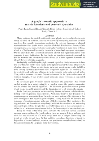
This thesis is concerned with the development of a novel technique to evaluate
matrix functions and its applications to the simulation of quantum dynamics. In
this chapter we present the motivations and origins of our approach and present an
outline of the thesis.
1.1 Simulating quantum systems
The quality of control over atomic systems in state of the art experiments is such that
one can now address and observe quantum evolutions of individual atoms in optical-
lattices [1, 2, 3, 4]. Additionally, coherent inter-atomic and light-matter interactions
can be made strong enough to occur on short time-scales compared to incoherent
processes. This reveals the system’s unitary evolution at the individual constituent
level which is of fundamental interest in the study of quantum many-body phenom-
ena. Several applications like quantum simulation and quantum computing schemes
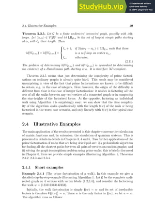
also rely on this information [5]. On the other hand, the theoretical simulation on a
classical computer of such non-equilibrium many-body dynamics is very challenging,
mainly due to the exponentially large number of relevant degrees of freedom.
Indeed, consider a “simple” quantum many-body systems comprising N motion-
less particles, each with 2 energy levels. Then a full description of the system wave-
function ψ requires 2N
complex numbers. This means that a direct exact solution
of Schrödinger’s equation, which describes the coherent dynamics of non-relativistic
quantum systems, is not accessible above N & 20. Even worse, for N & 250, this
number exceeds the number of atoms in the observable universe so even storing ψ on
a computer memory is impossible. For these reasons the problem of simulating the
time evolution of quantum many-body systems is believed to be intractable. Pon-
dering on this difficulty, R. Feynman proposed the idea of using quantum systems
to simulate other quantum systems, thereby turning the exponential scaling of ψ to
our advantage [6]. The validity of this idea was firmly established by S. Lloyd some
14 years later when he showed that universal quantum computation was possible [7].
This means that it is in principle possible to simulate any quantum system relying
1](https://image.slidesharecdn.com/agraphtheoreticapproachtomatrixfunctionsandquantumdynamicsphdthesis-230805203656-4458b8ad/85/A-Graph-Theoretic-Approach-To-Matrix-Functions-And-Quantum-Dynamics-PhD-Thesis-11-320.jpg)
![2 Introduction
on a few universal quantum operations. The same year A. Steane presented the first
quantum error correcting code [8], demonstrating that quantum computation was
not fundamentally impaired by decoherence. Finally the recognition that quantum
computers could efficiently solve problems beyond the scope of classical comput-
ers [9, 10] initiated a strong research effort toward physical realisation of quantum
computers.
In the mean time, nothing precludes in principle the existence of a small set
of parameters, whose cardinality scales polynomially with N, and from which one
could construct a good description of ψ. This observation in conjunction with the
recent experimental advances has led to the rise of an active area of research focused
on the development of theoretical methods to approximate the coherent dynamics of
quantum systems. Among the most well known techniques are the Density Matrix
Renormalisation Group method [11], related Tensor Network approaches [12] and
the Time-Evolving Block Decimation method [13]. These techniques have proven
very successful in their respective domains of applicability (e.g. [14, 15, 16]), i.e.
mostly 1D systems with nearest neighbour interactions. On the contrary, and in
spite of extensive work in the field, very few techniques exist in 2D and 3D [17, 18]
and for systems exhibiting long-range interactions.
As part of this ongoing effort, we develop in this thesis a new technique which
aims at simulating the coherent time dynamics of quantum systems, termed path-
sum, and which is not limited by the system geometry. This technique is based on
novel results concerning the algebraic structure of sets of walks on graphs. Below,
we explain the origins of this approach.
1.2 Of graphs and matrices
The “most basic result of algebraic graph theory” [19] states that the powers of the
adjacency matrix of a graph generate all the walks on this graph [20]. This extends
to weighted graphs, with matrix powers giving the sum of the weights of the walks
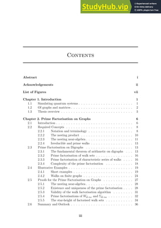
on the graph [19]. To clarify these notions, consider the following example:
A =
a11 a12
a21 a22
−→ (A3
)11 = a3
11
|{z}
+ a12a22a21
| {z }
+ a12a21a11
| {z }
+ a11a12a21
| {z }
1
2
Each term contributing to (A3
)11 can be seen as the weight of a walk whose trajectory
we read off the subscripts. For example, a11a12a21 is the weight of the walk w : 1 →
2 → 1 → 1, which is illustrated above. Note how the ordering of the walk (left-to-
right) differs from the ordering of the weights (right-to-left). In this representation,
individual entries of the matrix A represent the weight of an edge of the graph, e.g.
a12 is the weight of the edge from vertex 2 to vertex 1. The weight of a walk is then
the product of the weights of the edges it traverses.](https://image.slidesharecdn.com/agraphtheoreticapproachtomatrixfunctionsandquantumdynamicsphdthesis-230805203656-4458b8ad/85/A-Graph-Theoretic-Approach-To-Matrix-Functions-And-Quantum-Dynamics-PhD-Thesis-12-320.jpg)
![1.3. Thesis overview 3
The fundamental equivalence between walks on graphs and matrix powering
illustrated above, bore many fruits over the years, in particular in combinatorics
[19, 21, 22] and probability theory [23, 24]. In quantum mechanics, it manifests
itself most simply through Schrödinger’s equation. This equation is
H|ψ(t)i = i~
d
dt
|ψ(t)i,
where ~ is the reduced Planck constant, |ψ(t)i is a vector describing the instan-
taneous state of the system at time t written here in Dirac notation and H is the
Hamiltonian matrix, a representation of the system energy, which we shall always
consider to be finite and discrete. The Schrödinger equation is formally solved by
the matrix exponential U(t) = exp(−iHt/~) and |ψ(t)i = U(t)|ψ(0)i. The matrix
exponential U(t) has a power series representation which naturally involves powers
of the Hamiltonian Hn
, n ≥ 0. By virtue of the equivalence between walks and
matrix powers, the matrix exponential U(t) is thus seen to be equivalent to a series
of walks.
The observation underlying this thesis is that if sets of walks can be endowed
with an algebraic structure such that there exists a small set of objects generating all
the walks, then one might accelerate the convergence of a walk series by expressing
it using these generators. By the equivalence between walks and matrix powers, this
would in turn imply novel representations for functions of matrices, and in particular
for the matrix exponential U(t) which describes the dynamics of quantum systems.
This is what we achieve in the thesis.
1.3 Thesis overview
The thesis is organised as follows. We begin in Chapter 2 by constructing an al-
gebraic structure for sets of walks on arbitrary finite graphs. In particular, we
demonstrate that all the walks factorise uniquely into nesting products of prime
walks. Nesting is a product operation between walks which we introduce. It follows
that these primes are the generators of all walks. By factoring sets of walks into
products of sets of primes, we obtain a recursive formula which describes the set of
all walks using only the prime generators. Thanks to this result we derive a universal
continued fraction representation for the formal series of all walks between any two
vertices of a graph. We give illustrating examples and applications for these results.
In Chapter 3 we present the main application of the prime factorisation of walks:
the method of path-sums. By relying on the correspondence between matrix multi-
plications and walks on graphs, we show that any primary matrix function f(M) of
a finite matrix M can be expressed solely in terms of the prime walks sustained by
a graph G describing the sparsity structure of M. We give explicit formulae for the
matrix raised to a complex power, the matrix exponential, the inverse and the ma-
trix logarithm. We then provide examples and mathematical applications of these
results in the realm of matrix computations.](https://image.slidesharecdn.com/agraphtheoreticapproachtomatrixfunctionsandquantumdynamicsphdthesis-230805203656-4458b8ad/85/A-Graph-Theoretic-Approach-To-Matrix-Functions-And-Quantum-Dynamics-PhD-Thesis-13-320.jpg)

![Chapter 2
Prime Factorisation on Graphs
Everyone engaged in research must have had the experience of working
with feverish and prolonged intensity to write a paper which no one else
will read or to solve a problem which no one else thinks important and
which will bring no conceivable reward – which may only confirm a gen-
eral opinion that the researcher is wasting his time on irrelevancies.
N. Chomsky
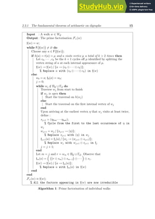
In this chapter we show that the formal series of all walks between any two
vertices of any finite digraph or weighted digraph G is given by a universal continued
fraction of finite depth involving the simple paths and simple cycles of G. A simple
path is a walk forbidden to visit any vertex more than once, a simple cycle is a
cycle whose internal vertices are all distinct and different from the initial vertex.
We obtain an explicit formula giving this continued fraction. Our results are based
on an equivalent to the fundamental theorem of arithmetic: we demonstrate that
arbitrary walks on G uniquely factorise into nesting products of simple paths and
simple cycles. Nesting is a walk product which we define. We show that the simple
paths and simple cycles are the prime elements of the set of all walks on G equipped
with the nesting product. We give an algorithm producing the prime factorisation of
individual walks. We obtain a recursive formula producing the prime factorisation
of sets of walks.
The work in this chapter forms the basis of an article that is currently under
review for publication in Forum of mathematics Sigma, Cambridge University Press.
2.1 Introduction
Walks on graphs are pervasive mathematical objects that appear in a wide range
of fields from mathematics and physics to engineering, biology and social sciences
[22, 19, 25, 26, 27, 28, 29]. Walks are perhaps most extensively studied in the
context of random walks on lattices [30], e.g. because they model physical processes
[31]. At the same time, it is difficult to find general ‘context-free’ results concerning
walks and their sets. Indeed, properties obeyed by walks are almost always strongly
dependent on the graph on which the walks take place. For this reason, many
results concerning walks on graphs are dependent on the specific context in which
they appear.
6](https://image.slidesharecdn.com/agraphtheoreticapproachtomatrixfunctionsandquantumdynamicsphdthesis-230805203656-4458b8ad/85/A-Graph-Theoretic-Approach-To-Matrix-Functions-And-Quantum-Dynamics-PhD-Thesis-16-320.jpg)
![2.1. Introduction 7
In this chapter, we study walks and their sets on digraphs and weighted digraphs
as separate mathematical entities and with minimal context. We demonstrate that
they obey non-trivial properties that are largely independent of the digraph on
which the walks take place. Foremost amongst these properties is the existence and
uniqueness of the factorisation of walks into products of primes, which we show are
the simple paths and simple cycles of the digraph, also known as self-avoiding walks
and self-avoiding polygons, respectively. Another such property is the existence of a
universal form for the formal series of all walks between any two vertices of any finite
(weighted) digraph: it is a continued fraction of finite depth, which we provide. This
universal continued fraction has already found applications in the fields of matrix
functions and quantum dynamics, which we present in Chapters 3, 4 and 5. We
believe that the unique factorisation property will also find applications in the field
of graph characterisation as we show in Chapter 6. Indeed, a digraph is, up to an
isomorphism, uniquely determined by the set of all walks on it [32]. The prime
factorisation of walk sets which we provide will reduce the difficulty of comparing
walk sets to comparing sets of primes, of which there is only a finite number on any
finite digraph.
Usually, the product operation on the set WG of all walks on a digraph G is
the concatenation. It is a very liberal operation: the concatenation a ◦ b of two
walks is non-zero whenever the final vertex of a is the same as the initial vertex of
b. This implies that both the irreducible and the prime elements of the set of all
walks equipped with the concatenation product, denoted (WG, ◦), are the walks of
length 1, i.e. the edges of G. Consequently, the factorisation of a walk w on G into
concatenations of prime walks is somewhat trivial. For this reason, we abandon the
operation of concatenation and introduce instead the nesting product, symbol ⊙,
as the product operation between walks on G. Nesting is a much more restrictive
operation than concatenation, in that the nesting of two walks is non-zero only if
the walks satisfy certain constraints. As a result of these constraints, the irreducible
and prime elements of (WG, ⊙), obtained upon replacing the concatenation with the
nesting product, are the simple paths and simple cycles of G, rather than its edges.
The rich structure that is consequently induced on walk sets is at the origin of the
universal continued fraction formula for formal series of walks.
This chapter is organised as follows. In §2.2, we present the notation and ter-
minology used throughout the chapter. In particular we define the nesting product
and establish its properties in §2.2.2. In §2.3 we give the main results of the present
chapter: (i) existence and uniqueness of the factorisation of any walk into nesting
products of primes, the simple paths and simple cycles; (ii) an algorithm produc-
ing the prime factorisation of individual walks; (iii) a recursive formula factorising
walk sets into nested sets of primes; (iv) a universal continued fraction representing
factorised formal series of walks on digraphs and weighted digraphs; and (v) identi-
fication of the depth of this continued fraction with the length of the longest prime.
The results of this section are proven in sections 2.5.2, 2.5.3 and 2.5.4. Finally, in
§2.4 we present examples illustrating our results.](https://image.slidesharecdn.com/agraphtheoreticapproachtomatrixfunctionsandquantumdynamicsphdthesis-230805203656-4458b8ad/85/A-Graph-Theoretic-Approach-To-Matrix-Functions-And-Quantum-Dynamics-PhD-Thesis-17-320.jpg)
![2.2.1 Notation and terminology 9
Let V = {V } be a collection of vector spaces, each of arbitrary finite dimension,
such that V is in one to one correspondence with the vertex set V(G) of a finite
directed graph G. For simplicity we designate by Vµ ∈ V the vector space associated
to vertex µ ∈ V(G). Let F = {ϕµ→ν : Vµ → Vν} be a collection of linear mappings
in one to one correspondence with the edge set E(G) of G. We associate the linear
mapping ϕν←µ ∈ F to the directed edge from µ to ν. Then G = (V, F) is a
representation of the directed graph G, which in this context is also called a quiver
[33, 34]. The representation of a walk w = (α1α2 · · · αℓ) ∈ WG is the linear mapping
ϕw obtained from the composition of the linear mappings representing the successive
edges traversed by the walk ϕw = ϕαℓ←αℓ−1
◦· · ·◦ϕα3←α2 ◦ϕα2←α1 . The representation
of a trivial walk (µ) is the identity map 1µ on Vµ and the representation of the empty
walk 0 is the 0 map.
Remark 2.2.2. The utility of the quiver as a representation of a digraph is explained
in Remark 2.2.5, p. 12.
A weighted digraph (G, W) is a digraph G paired with a weight function W that
assigns a weight W[e] to each directed edge e of G. We let the weight of a directed
edge from µ to ν, denoted wνµ = W[(µν)], be a dν-by-dµ complex matrix representing
the linear mapping ϕν←µ. Furthermore, we impose that W[0] = 0 and W[(µ)] = Iµ,
the identity matrix of dimension dµ. For two directed edges e1 and e2 such that
e1 ◦ e2 6= 0, we let
W[e1 ◦ e2] = W[e2]W[e1]. (2.2)
Note that the ordering of the weights when two edges are concatenated is suitable for
the multiplication of their weights to be carried out. The weight of a walk w ∈ WG,
denoted W[w], is the right-to-left product of the weights of the edges it traverses.
Since walks are in one to one correspondence with linear mappings, for any two
walks w, w′
satisfying h(w) = h(w′
) and t(w) = t(w′
) we define the sum w + w′
as
the object whose representation is the linear mapping which is sum of the two linear
maps representing w and w′
, ϕw+w′ = ϕw + ϕw′ . It follows that
W
w + w′
= W
w
+ W
w′
. (2.3)
We require the empty walk to be the neutral element of the addition operation +,
i.e. w + 0 = w and W
w + 0
= W[w].
The characteristic series of WG; αω is the formal series [35]
ΣG; αω =
X
w∈WG; αω
w. (2.4)
In other words, the coefficient of w in ΣG; αω, denoted (ΣG; αω, w), is 1 if w ∈ WG; αω
and 0 otherwise. If it exists, the weighted characteristic series W[ΣG; αω] is the series
of all walk weights.
Remark 2.2.3 (More general weights). It is possible to generalise the definitions
of quiver and of weighted digraph to the case where the weight of an edge from µ](https://image.slidesharecdn.com/agraphtheoreticapproachtomatrixfunctionsandquantumdynamicsphdthesis-230805203656-4458b8ad/85/A-Graph-Theoretic-Approach-To-Matrix-Functions-And-Quantum-Dynamics-PhD-Thesis-19-320.jpg)
![10 Prime Factorisation on Graphs
=
J J
a1
a2
a3
a4
a5
a6
a7
a8
a9
a1
a2
a3
a4 a4
a5
a6
a7 a7
a8
a9
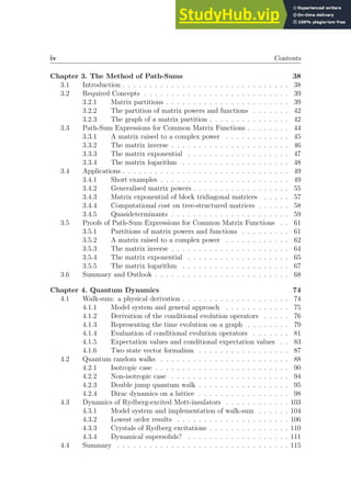
w p c1 c2
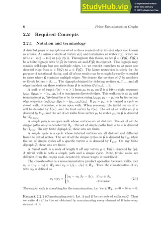
Figure 2.1: An example of nesting: the walk w = α1α2α3α4α5α6α7α8α9α7α4 is
obtained upon inserting the simple cycle c2 = α7α8α9α7 into c1 = α4α5α6α7α4 and
then into the simple path p = α1α2α3α4, that is w = p ⊙ c1 ⊙ c2
.
to ν is any morphism φν←µ : Vµ → Vν in an additive category C from an object Vµ,
associated with the vertex µ, to an object Vν, associated with the vertex ν. Then
all the results of this chapter hold upon requiring that the matrix of morphisms
(M)νµ = φν←µ be invertible. This remark is based on an observation of [36].
2.2.2 The nesting product
We now turn to the definition and properties of the nesting product. Nesting is
more restrictive than concatenation; in particular, the nesting of two walks will be
non-zero only if they obey the following property:
Definition 2.2.1 (Canonical property). Consider (a, b) ∈ W2
G with b = β β2 · · · βq β
a cycle off β, and a = α1 α2 · · · β · · · αk a walk that visits β at least once. Let αj = β
be the last appearance of β in a. Then the couple (a, b) is canonical if and only if
one of the following conditions holds:
(i) a and b are cycles off the same vertex β; or
(ii) {αij 6= β} ∩ b = ∅; that is, no vertex other than β that is visited by a before
αj is also visited by b.
Definition 2.2.2 (Nesting product). Let (w1, w2) ∈ W2
G . If the couple (w1, w2)
is not canonical, we define the nesting product to be w1 ⊙ w2 = 0. Otherwise, let
w1 = (η1 η2 · · · β · · · ηℓ1 ) be a walk of length ℓ1 and let w2 = (β κ2 · · · κℓ2 β) be a cycle
of length ℓ2 off β. Then the operation of nesting is defined by
⊙ : WG × WG → WG, (2.5a)
(w1, w2) → w1 ⊙ w2 = (η1 η2 · · · β κ2 · · · κℓ2 β · · · ηℓ1 ). (2.5b)
The walk w1 ⊙w2 of length ℓ1 +ℓ2 is said to consist of w2 nested into w1. The vertex
sequence of w1 ⊙ w2 is formed by replacing the last appearance of β in w1 by the
entire vertex sequence of w2.
◮ Nesting is non-commutative and non-associative: for example, 11 ⊙ 131 = 1131,
while 131 ⊙ 11 = 1311, and 12 ⊙ 242
⊙ 11 = 11242, while 12 ⊙ 242 ⊙ 11
= 0.](https://image.slidesharecdn.com/agraphtheoreticapproachtomatrixfunctionsandquantumdynamicsphdthesis-230805203656-4458b8ad/85/A-Graph-Theoretic-Approach-To-Matrix-Functions-And-Quantum-Dynamics-PhD-Thesis-20-320.jpg)
![2.2.3 The nesting near-algebra 11
◮ Nesting coincides with concatenation for cycles off the same vertex. Let (c1, c2) ∈
W2
G; αα, then c1 ⊙ c2 = c1 ◦ c2. Consequently nesting is associative over the cycles,
(c1 ⊙ c2) ⊙ c3 = c1 ⊙ (c2 ⊙ c3) = c1 ⊙ c2 ⊙ c3 where c3 ∈ WG; αα. This in turn implies
power-associativity over the cycles and we simply write cp
for the nesting of a cycle
c with itself p times, e.g. 1212121 = 121 ⊙ 121 ⊙ 121 = 1213
. We interpret c0
as the
trivial walk off h(c).
◮ Let µ ∈ V(G). Consider the trivial walk (µ) and observe that for any cycle w ∈ WG
visiting µ we have (µ) ⊙ w = w ⊙ (µ) = w. Therefore we say that a trivial walk is a
local identity element on the cycles. For any open walk w′
∈ WG visiting µ, we have
w′
⊙ (µ) = w′
and we say that a trivial walk is a local right-identity element on the
open walks.
Remark 2.2.4 (Nesting sets). Let A and B be two sets of walks on G. Then we
write A ⊙ B for the set obtained by nesting every element of B into every element
of A.
Definition 2.2.3 (Kleene star and nesting Kleene star). Let α ∈ V(G) and let
Eα ⊆ WG; αα. Set E0
α = {(α)} and Ei
α = Ei−1
α ◦ Eα for i ≥ 1. Then the Kleene
star of Eα, denoted E∗
α, is the set of walks formed by concatenating any number of
elements of Eα, that is E∗
α =
S∞
i=0 Ei
α [37]. The nesting Kleene star of Eα, denoted
E⊙∗
α , is the equivalent of the Kleene star with the concatenation replaced by the
nesting product: E⊙∗
α =
S∞
i=0 E⊙i
α where E⊙0
α = {(α)} and E⊙i
α = E
⊙(i−1)
α ⊙ Eα for
i ≥ 1. Since nesting coincides with concatenation for cycles off the same vertex, the
nesting Kleene star coincide with the usual Kleene star E⊙∗
α = E∗
α. Thus, from now
on we do not distinguish between the two.
Finally, with the nesting product comes a notion of divisibility. This notion plays
a fundamental role in the identification of irreducible and prime walks:
Definition 2.2.4 (Divisibility). Let (w, w′
) ∈ W2
G . We say that w′
divides w, and
write w′
| w, if and only if ∃ (a, b) ∈ W2
G such that either w = (a ⊙ w′
) ⊙ b or
w = a ⊙ (w′
⊙ b).
2.2.3 The nesting near-algebra
Having established the properties of the nesting product, we now turn to determining
the structure it induces on the sets of walks and their characteristic series. In order
for the latter to be defined, we need to equip walk sets with an addition. To this
end, and in the spirit of the path algebra KG [38], we want to construct a K-algebra
with the set of walks WG as basis but equipped with the nesting product instead of
the concatenation. However left-distributivity of the nesting product with respect
to addition does not hold (§2.5.1). Therefore, we define instead a near K-algebra
equipped with the nesting product.
Definition 2.2.5 (Near K-algebra [38]). Let K be an algebraic closed field and A a
set. Let + and • be an addition and a product operation defined between elements](https://image.slidesharecdn.com/agraphtheoreticapproachtomatrixfunctionsandquantumdynamicsphdthesis-230805203656-4458b8ad/85/A-Graph-Theoretic-Approach-To-Matrix-Functions-And-Quantum-Dynamics-PhD-Thesis-21-320.jpg)
![2.2.4 Irreducible and prime walks 13
2.2.4 Irreducible and prime walks
We are now ready to identify the irreducible and prime elements of (WG, ⊙). Follow-
ing standard definitions [39, 40], a walk w ∈ WG is irreducible if, whenever ∃ a ∈ WG
with a | w, then either a is trivial, or a = w up to nesting with trivial walks (i.e. local
identities). In the opposite situation, we say that w is reducible. A walk w ∈ WG is
prime with respect to nesting if and only if for all (a, b) ∈ W2
G such that w | a ⊙ b
then w | a or w | b. The irreducible and prime elements of (WG, ⊙) are identified by
the following result:
Proposition 2.2.1. The set of irreducible walks is exactly ΠG ∪ΓG. The irreducible
walks are the prime elements of (WG, ⊙).
Remark 2.2.6 (Identifying the simple paths and simple cycles). The simple paths
and simple cycles of the digraph G can be systematically obtained via the powers
of its nilpotent adjacency matrix [41, 42]. The nilpotent adjacency matrix ĀG is
constructed by weighting the adjacency matrix A of G with formal variables ζe, one
for each directed edge e and such that: i) [ζe, ζe′ ] = 0 for any two edges (e, e′
) ∈ E(G);
and ii) ζ2
e = 0 for all edges e ∈ E(G). From this last property, it follows that only
the simple paths and simple cycles a non-zero coefficient in powers of ĀG.
We defer the proof of Proposition 2.2.1 to §2.5.2. Having established the def-
inition and properties of the nesting product as well as the irreducible and prime
elements it induces in (WG, ⊙), we turn to the factorisation of individual walks and
walk sets.
2.3 Prime Factorisation on Digraphs
In this section, we present the main results of this chapter. First, we present the
equivalent to the fundamental theorem of arithmetic on digraphs and we give an
algorithm factoring walks into nesting products of primes. Second, we give a formula
for factoring the set of walks WG; αω between any two vertices of G into nesting
products of sets of primes. Third, we give a universal form for the prime factorisation
of the characteristic series of all walks between any two vertices of any finite digraphs.
Fourth, we give an equivalent relation for weighted digraphs. As we will see, these
two universal forms are continued fractions of finite depth over the simple paths and
simple cycles of the digraph. Finally, we relate the depth of the continued fractions
with the length of the longest simple path. All the results of this section are proven
in §2.5.2–2.5.4 and examples illustrating their use are provided in §2.4.
2.3.1 The fundamental theorem of arithmetic on digraphs
The fundamental theorem of arithmetic is arguably the most important result in
the field of number theory [43]. It establishes the central role played by the prime
numbers and has many profound consequences on the properties of integers. We](https://image.slidesharecdn.com/agraphtheoreticapproachtomatrixfunctionsandquantumdynamicsphdthesis-230805203656-4458b8ad/85/A-Graph-Theoretic-Approach-To-Matrix-Functions-And-Quantum-Dynamics-PhD-Thesis-23-320.jpg)
![14 Prime Factorisation on Graphs
now present its analogue for individual walks on arbitrary digraphs. We begin by
stating the conditions under which two factorisations of a walk into nesting products
of shorter walks are equivalent.
Definition 2.3.1 (Factorisation of a walk). Let w ∈ WG. A factorisation of the
walk w, denoted f(w), is a way of writing w using nesting products of at least two
walks, called the factors.
Definition 2.3.2 (Equivalent factorisations). Let w ∈ WG. We say that two fac-
torisations f1(w) and f2(w) of a walk w are equivalent, denoted f1(w) ≡ f2(w), if and
only if one can be obtained from the other through the reordering of parentheses
and factors, and up to nesting with trivial walks, without modifying w. Equivalent
factorisations have the same non-trivial factors.
Definition 2.3.3 (Prime factorisation). A prime factorisation f̂(w) of a walk w ∈
WG is a factorisation of w into nesting products of simple paths and simple cycles.
The relation ≡ between factorisations of Definition 2.3.2 is clearly an equivalence
relation. Thus, for each walk w on G, it defines an equivalence class on the set of all
prime factorisations of this walk, Fw = {f̂(w)}. It is a central result of this chapter
that all prime factorisations of w belong to the same equivalence class [F⊙(w)] =
{f̂(w) ∈ Fw, f̂(w) ≡ F⊙(w)} and the set of irreducible factors of w is uniquely
determined by w:
Theorem 2.3.1 (Fundamental theorem of arithmetic on digraphs). Any walk on
G factorises uniquely, up to equivalence, into nesting products of primes, the simple
paths and simple cycles on G.
From now on we shall thus speak of the prime factorisation F⊙(w) of a walk w.
Below we give an algorithm that produces F⊙(w) for an arbitrary walk.
An algorithm to factorise individual walks
Let w ∈ WG and F f(w)
be the set of reducible factors appearing in a factorisation
f(w) of w.
Algorithm 1, presented on p. 15, picks an arbitrary reducible factor of a ∈
F f(w)
(initially we let f(w) = w) and factorises a into nesting products of strictly
shorter walks, yielding f(a). The algorithm then updates f(w), replacing a with
its factorisation in f(w), denoted f(w) → f(w) / {a → f(a)}. At this point, the
above procedure starts again, with the algorithm picking an arbitrary reducible
factor appearing in the updated factorisation f(w). At each round, reducible factors
are decomposed into nesting products of shorter walks. The algorithm stops when
F f(w)
is the empty set ∅, at which point f(w) is the prime factorisation F⊙(w) of
w. We demonstrate the validity of the algorithm in §2.5.3.
◮ A detailed example of the use of Algorithm 1 is provided in §2.4.1.](https://image.slidesharecdn.com/agraphtheoreticapproachtomatrixfunctionsandquantumdynamicsphdthesis-230805203656-4458b8ad/85/A-Graph-Theoretic-Approach-To-Matrix-Functions-And-Quantum-Dynamics-PhD-Thesis-24-320.jpg)
![2.3.3 Prime factorisation of characteristic series of walks 17
vertex representing the characteristic series of all the cycles that can be nested off
µ on the appropriate subgraph of G. Using the vertex-edge notation of walks, the
dressed vertex is therefore
(α)′
G =
X
p∈N
X
(αµ2···µmα) ∈ ΓG; α
(α)(αµ2)(µ2)′
G{α} · · · (µm)′
G{α, µ2,··· ,µm−1}(µmα)(α)
p
,
=
X
p∈N
X
γ∈ΓG; α
γ′
p
, (2.8)
where the sums over p ∈ N account for cycles made of a single repeated simple cycle,
e.g. γp
, and γ′
is a notation for a simple cycle γ with dressed vertices. Finally, we
show in §2.5.4 that the linear mapping representing a dressed vertex on the quiver
is the inverse mapping ϕ(α)′
G
= 1α −
P
γ∈ΓG; α
ϕγ′
−1
and from now on we represent
dressed vertices using the inverse notation.
Theorem 2.3.3 (Path-sum). Let ΣG; αω denote the characteristic series of all walks
from α to ω on G. Then ΣG; αω is given in vertex-edge notation by
ΣG; αω =
X
ΠG; αω
(α)′
G (αν2) (ν2)′
G{α} · · · (νpω) (ω)′
G{α,ν2,...,νp} , (2.9a)
where p is the length of the simple path (αν2 · · · νpω) ∈ ΠG; αω, and (α)′
G denotes the
dressed vertex α on G, given by
(α)′
G =
(α) −
X
ΓG; α
(α) (αµ2) (µ2)′
G{α} (µ2µ3) · · · (µm)′
G{α,µ2,...,µm−1} (µmα) (α)
#−1
,
(2.9b)
where m is the length of the simple cycle (αµ2 · · · µmα) ∈ ΓG; α.
The dressed vertex (α)′
G is defined recursively through Eq. (2.9b) since it is
expressed in terms of dressed vertices (µj)′
G{α,µ2,...,µj−1}. These are in turn de-
fined through Eq. (2.9b) but on the subgraph G{α, µ2, . . . , µj−1} of G. The re-
cursion stops when vertex µj has no neighbour on this subgraph, in which case
(µj)′
G{α,µ2,...,µj−1} = [(µj)−(µjµj)]−1
if the loop (µjµj) exists and (µj)′
G{α,µ2,...,µj−1} =
(µj) otherwise.
The recursive definition of dressed vertices implies that the formula of Theorem
2.3.3 for ΣG; αω yields a formal continued fraction. On finite digraphs, the depth
of this continued fraction is finite, see §2.3.4. The formal factorisation of ΣG; αω
achieved by Theorem 2.3.3 yields a factorised form for series of walks on weighted
digraphs. This directly leads to applications in the field of matrix computations, as
shown in the next chapter.](https://image.slidesharecdn.com/agraphtheoreticapproachtomatrixfunctionsandquantumdynamicsphdthesis-230805203656-4458b8ad/85/A-Graph-Theoretic-Approach-To-Matrix-Functions-And-Quantum-Dynamics-PhD-Thesis-27-320.jpg)
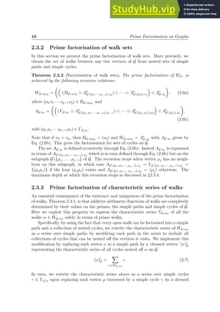
![18 Prime Factorisation on Graphs
Theorem 2.3.4 (Weighted path-sum). Let M be an invertible matrix defined through
(M)νµ = wνµ. Then as long as all of the required inverses exist, the weight of the
sum of all walks from α to ω on the weighted digraph (G, W) is given by
W
ΣG; αω
=
X
ΠG; αω
FG{α,...,νp}; ω wωνp · · · FG{α}; ν2 wν2α FG;α , (2.10a)
where p is the length of the simple path, wνµ = W[(µν)] is the weight of the edge
(µν), and
FG; α ≡ W
(α)′
G
=
Iµ −
X
ΓG; α
wαµm FG{α,...,µm−1}; µm wµmµm−1 · · · FG{α}; µ2 wµ2α
−1
,
(2.10b)
with m the length of the simple cycle and Iµ the dµ × dµ identity matrix. FG; α is the
effective weight of the vertex α on G once it is dressed by all the cycles off it.
The expression of W
ΣG; αω
is a continued fraction of finite depth, which results
from the recursive definition of the FG; α. Theorem 2.3.4 thus expresses the sum of
the weights of all walks from α to ω on any finite digraph as a finite matrix-valued
continued fraction over the simple paths and simple cycles of G. As we will see
with the examples, this allows direct verifications using matrix computations of the
results of Theorem 2.3.3 and 2.3.4, which look otherwise very abstract. But before
we give examples illustrating the Theorems above, we determine the depth at which
the continued fraction terminates.
2.3.4 Complexity of the prime factorisation
The prime factorisation of a walk set WG; αω reduces this set to nested sets of prime
walks. Since these primes – the simple cycles and simple paths of G – are difficult
to identify, we expect the factorised form of WG;αω to be difficult to construct. For
example, if the digraph is Hamiltonian, the Hamiltonian cycle or path must appear
in the factorisation of at least one walk set. Consequently, we expect that factoring
all the walk sets requires determining the existence of such a cycle or path, a problem
which is known to be NP-complete.
In order to formalise this observation, we now determine the star-height of the
prime factorisation, as given by Theorem 2.3.2, of any set WG; αω. The star-height
h(E) of a regular expression E was introduced by Eggan [44] as the number of nested
Kleene stars in E. This quantity characterises the structural complexity of formal
expressions. As we will see in the examples of §2.4, prime factorisations of walk
sets typically have a non-zero star-height. Furthermore, the proofs of Theorems
2.3.3 and 2.3.4 in §2.5.4 demonstrate that the star-height of WG; αω is equal to the
depth of the continued fraction generated by Theorems 2.3.3 and 2.3.4. In §2.5.5
we obtain an exact recursive expression for h(WG; αω). The following result says
that the problem of evaluating h(WG; αω) is nonetheless NP-complete on undirected
connected graphs:](https://image.slidesharecdn.com/agraphtheoreticapproachtomatrixfunctionsandquantumdynamicsphdthesis-230805203656-4458b8ad/85/A-Graph-Theoretic-Approach-To-Matrix-Functions-And-Quantum-Dynamics-PhD-Thesis-28-320.jpg)
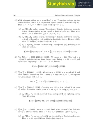
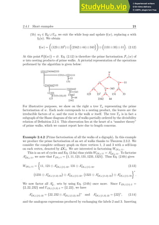
![2.4.1 Short examples 23
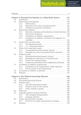
1
2
3
4
6
5
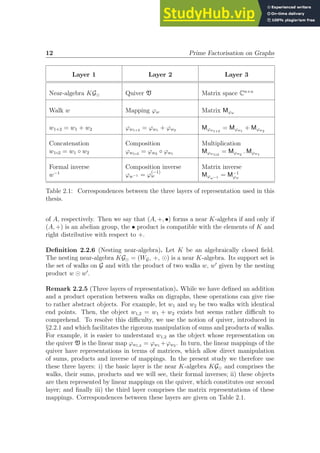
Figure 2.2: The digraph G of Example 2.4.4.
by following the procedure described in the proof of Theorem 2.3.3: we sum the
elements of the factorised form of WK3; 11, with the sums over the Kleene stars
yielding formal inverses.
The best way to convince oneself of the correctness of the prime factorisation of
a characteristic series such as Eq. (2.18) is to give weights to the graph edges. In
this situation, and if the factorisation is correct, the weight of the continued fraction
representing the prime factorisation of the characteristic series is directly identifiable
with a matrix inverse. This inverse can often be calculated through direct matrix
computations, allowing a direct verification of the factorisation. This is what we
show in the next example.
Example 2.4.4 (Walk generating function). Consider the digraph G illustrated on
Fig. 2.2, and let A be its adjacency matrix. Let gG; 11(z) =
P∞
n=0 zn
(An
)11 be the
walk generating function for all the walks on G from vertex 1 back to itself [20]. This
can be computed by noting that g11(z) is the sum of the weights of all the walks
w ∈ WG; 11 on a weighted version of G, which has an edge weight of z assigned to
every edge.
Theorem 2.3.3 yields ΣG; 11, the sum of all walks on the unweighted digraph G, as
ΣG; 11 =
h
(1) − (11) − (12)(2)′
G{1}(231)
i−1
, (2.20a)
(2)′
G{1} =
h
(2) − (24)(4)′
G{1,2}(42)
i−1
, (4)′
G{1,2} =
h
(4) − (44) − (4564)
i−1
,
(2.20b)
which corresponds to summing over the factorised form
WG; 11 =
n
11, 1231 ⊙
242 ⊙ {44, 4564}∗ ∗
o∗
. (2.21)
According to Theorem 2.3.4, the sum over the walks of the weighted digraph is
obtained upon replacing each edge by its weight in Eq. (2.20). This yields
W
ΣG; 11
=
1
1 − z − z 1
1−z 1
1−z−z3 z
z2
= −
z3
+ z2
+ z − 1
z6 + 2z4 − z3 − 2z + 1
. (2.22)
We can verify that W
ΣG; 11
is equal to gG; 11(z) = [I − zA]−1
)11, where I is the
6 × 6 identity matrix, provided |z| ρ(A)−1
with ρ(A) the spectral radius of A, as](https://image.slidesharecdn.com/agraphtheoreticapproachtomatrixfunctionsandquantumdynamicsphdthesis-230805203656-4458b8ad/85/A-Graph-Theoretic-Approach-To-Matrix-Functions-And-Quantum-Dynamics-PhD-Thesis-33-320.jpg)
![24 Prime Factorisation on Graphs
expected [20]. This shows that all the walks off 1 on G are indeed present in the
factorised form of the walk set Eq. (2.21) and that the prime factorisation of the
characteristic series Eq. (2.20) is correct.
Sometimes, the required matrix inverse is too complicated to be calculated, e.g.
because the matrix is too large or very ill-behaved such as nearly singular. In these
situations, the continued fraction representing the factorised characteristic series of
weighted walks is a reliable way of obtaining the matrix inverse. This observation
forms the basis of Chapter 3.
2.4.2 Walks on finite graphs
In this section we give a further example of application of Theorem 2.3.4: we obtain
the walk generating functions of finite Cayley trees. To this end, we first determine
the walk generating functions of finite path-graphs and cycle-graphs1
.
Walks on finite path-graphs and cycle graphs
Let Pn and Cn be the n-vertices undirected path-graph and cycle graph, respectively.
We are interested in their walk generating functions
gG; αω(z) =
X
n
|WG; αω;n|zn
, (2.23)
where |WG; αω;n| is the number of walks of length n from vertex α to vertex ω on G.
For convenience, we label the vertices of Pn from left to right, from 0 to n − 1.
Let α be a vertex of Pn, if α 6= 0, n − 1, then the only simple cycles off α on Pn
are the two back-tracks (α α ± 1 α) with weight z2
and, if α = 0 or n − 1, then only
one back-track exists. According to Theorem 2.3.4, the path-sum for gG; αα(z) thus
reads
gG; αα(z) =
1
1 − z2Fα(z) − z2Fn−α−1(z)
, (2.24)
where Fα is the continued fraction of depth α−1 which represents the weight of the
dressed neighbour of α,
Fα(z) = W
(α − 1)′
Pn{α}
=
1
1 − z2
1− z2
...
=
Qα−1(z)
Qα(z)
, (2.25)
with Qx(u) = 2F1
1
2
− x
2
, −x
2
; −x; 4u2
the Gauss hypergeometric function. Then,
gPn; αα(z) =
Qn−α−1(z)Qα(z)
Qn(z)
, (2.26)
1
Contrary to the generating functions of finite Cayley trees, those of finite path-graphs and
cycle-graphs are already known thanks to direct diagonalisation. We derive them again to illustrate
our results.](https://image.slidesharecdn.com/agraphtheoreticapproachtomatrixfunctionsandquantumdynamicsphdthesis-230805203656-4458b8ad/85/A-Graph-Theoretic-Approach-To-Matrix-Functions-And-Quantum-Dynamics-PhD-Thesis-34-320.jpg)
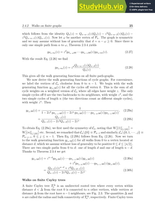
![26 Prime Factorisation on Graphs
Figure 2.3: Illustration of three finite Cayley trees with, from left to right, T 5
3 , T 4
4
and T 3
5 . The corresponding Bethe lattices are infinite in the radial direction.
and their infinite counterparts, the Bethe lattices Bn ≡ T ∞
n , have found widespread
applications in mathematics, physics and even in biology [45, 46, 47, 48].
Even though the finite Cayley tree appears at least as often as the infinite Bethe
lattice in applications, the former is usually approximated by the latter which is
easier to handle. Indeed, the walk generating functions of the Bethe lattices satisfy
easily solvable relations2
gBn; 00(z) = 1 − n z2
gBn{0}; 11(z)
−1
, (2.31a)
gBn{0}; 11(z) = 1 − (n − 1) z2
gBn{0}; 11(z)
−1
, (2.31b)
where 0 and 1 designate any vertex and any vertex neighbouring 0, respectively.
These equations are not fulfilled by finite Cayley trees, which exhibit finite size
effects that are often neglected for the sake of simplicity. Yet these effects are
generally important due to the large fraction of vertices on the outer-rim of the tree.
In this section we obtain the exact walk generating functions on any finite Cayley
tree.
We begin with the walk generating function gT ∆
n ; 00 for the cycles off the root of
the tree. There are n backtracks off the root of the tree with weight z2
and therefore
gT ∆
n ; αα =
1
1 − nz2F∆ z
√
n − 1
, (2.32)
with F∆ the finite continued fraction of depth ∆ defined in Eq. (2.25). Indeed, since
there are n − 1 backtracks off the neighbours of the roots on T ∆
n {0}, F∆ fulfills the
recursion relation
F∆ z
√
n − 1
=
1
1 − z2(n − 1)F∆−1 z
√
n − 1
, (2.33)
with solution F∆ z
√
n − 1
= Q∆−1 z
√
n − 1
/Q∆ z
√
n − 1
. The walk generating
2
Called self-consistency relations in the physics literature.](https://image.slidesharecdn.com/agraphtheoreticapproachtomatrixfunctionsandquantumdynamicsphdthesis-230805203656-4458b8ad/85/A-Graph-Theoretic-Approach-To-Matrix-Functions-And-Quantum-Dynamics-PhD-Thesis-36-320.jpg)
![28 Prime Factorisation on Graphs
algebra. We then prove the results of §2.3 on the prime factorisation of walks.
2.5.1 The nesting near-algebra
For (WG, +, ⊙) to form a noncommutative nonassociative near K-algebra, we must
verify that (WG, +) is an abelian group, shown in [38], and that the nesting product
is compatible with the scalars and right distributive.
Compatibility with the scalars: let (k1, k2) ∈ K2
, a ∈ WG; αω and b ∈ WG; µµ.
We show that (k1 a) ⊙ (k2 b) = k1k2(a ⊙ b). If a ⊙ b = 0 the property is trivially
true. Otherwise, according to Definition 2.2.2, ∃! a1 ∈ WG; αµ, ∃! a2 ∈ WG; µω with
a ⊙ b = a1 ◦ b ◦ a2. Then (k1 a) ⊙ (k2 b) = k1a1 ◦ (k2b) ◦ a2. Since concatenation is
bilinear, k1a1 ◦ (k2b) ◦ a2 = k1k2 (a1 ◦ b ◦ a2) = k1k2(a ⊙ b) and nesting is compatible
with the scalars.
Right-distributivity : let (a, b) ∈ W2
G; µµ and c ∈ WG; αω. We show that c ⊙ (a +
b) = c ⊙ a + c ⊙ b. Walks a and b being cycles off the same vertex µ (otherwise
a + b = 0 and the property is trivially true), it follows that c ⊙ a = 0 ⇐⇒ c ⊙ b =
0 ⇐⇒ c ⊙ (a + b) = 0 and the property is true as soon as c ⊙ a or b = 0.
Otherwise, definition 2.2.2 implies that ∃! c1 ∈ WG; αµ and ∃! c2 ∈ WG; µω such that
c ⊙ a = c1 ◦ a ◦ c2 and c ⊙ b = c1 ◦ b ◦ c2. Since concatenation is bilinear we have
c ⊙ a + c ⊙ b = c1 ◦ a ◦ c2 + c1 ◦ b ◦ c2 = c1 ◦ (a + b) ◦ c2 = c ⊙ (a + b) and nesting is
right distributive.
Failure of left-distributivity : let (a, b) ∈ W2
G; αω and c ∈ WG; µµ. We show that
in general (a + b) ⊙ c 6= a ⊙ c + b ⊙ c. Suppose that both a and b visit µ. Then
by Definition 2.2.2, ∃! a1 ∈ WG; αµ and ∃! a2 ∈ WG; µω with a ⊙ c = a1 ◦ c ◦ a2.
Similarly, b ⊙ c 6= 0 ⇒ ∃! b1 ∈ WG; αµ and ∃! b2 ∈ WG; µω with b ⊙ c = b1 ◦ c ◦ b2. Now
a ⊙ c + b ⊙ c = a1 ◦ c ◦ a2 + b1 ◦ c ◦ b2 6= (a1 + b1) ◦ c ◦ (a2 + b2) = (a + b) ⊙ c.
The nesting product is therefore compatible with the scalars and right-distributive
with respect to + but not left-distributive. It follows that KG⊙ = (WG, +, ⊙) is a
noncommutative nonassociative near K-algebra.
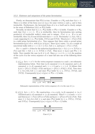
2.5.2 Existence and uniqueness of the prime factorisation
We begin by showing that the factorisation of a walk into nesting products of sim-
ple paths and simple cycles always exists and is unique in the sense of Definition
2.3.2. We then demonstrate Proposition 2.2.1, i.e. that the simple paths and simple
cycles are the prime elements of (WG, ⊙), thereby establishing Theorem 2.3.1 as an
equivalent to the fundamental theorem of arithmetic.
Let P(n) be the following proposition: ∀w ∈ WG of length ℓ(w) ≤ n, there exists
a unique factorisation, up to equivalence, of w into nesting products of irreducible
walks, i.e. ∃! F(w) ∈ Fw/ ≡.
We demonstrate that P(n) holds for all n ≥ 1 by induction on the walk length n.](https://image.slidesharecdn.com/agraphtheoreticapproachtomatrixfunctionsandquantumdynamicsphdthesis-230805203656-4458b8ad/85/A-Graph-Theoretic-Approach-To-Matrix-Functions-And-Quantum-Dynamics-PhD-Thesis-38-320.jpg)
![2.5.4 Prime factorisations of WG; αω and ΣG; αω 33
◮ We prove Theorem 2.3.3.
Proof. The theorem follows from Theorem 2.3.2. Consider WG; αω be the set of walks
from α to ω. We first decompose WG; αω using Eq. (2.6a), identifying α with ν0 and
ω with νp for convenience, then sum over the elements of the sets on both sides of
the equality. This yields, in vertex-edge notation,
ΣG; αω =
X
(αν1···νp−1ω)∈ΠG; αω
X
a0∈A∗
G; α
a0
(αν1)
X
a1∈A∗
G{α}; ν1
a1
(ν1ν2) · · · (2.44)
· · · (νp−1ω)
X
ap∈A∗
G{α,ν1,··· ,νp−1}; ω
ap
,
which we obtain upon nesting the sets A∗
G; α, A∗
G{α}; ν1
, . . . into the simple paths of
ΠG; αω at the appropriate positions. Equation (2.44) shows that the sums over these
sets can be seen as effective vertices produced by dressing each vertex of the simple
paths by all the cycles that visit these vertices on progressively smaller digraphs
G, G{α}, . . .. For example, we define a dressed vertex (α)′
G representing the series
of all the cycles off α on G as
(α)′
G =
X
a0∈A∗
G; α
a0. (2.45)
It follows that Eq. (2.44) yields Eq. (2.9a), with dressed vertices representing the
characteristic series of the A∗
G{α,ν1···νj−1}; νj
sets. These series are proper [49]: their
constant term is a trivial walk, e.g. (α) in Eq. (2.45), which is different from the
empty walk 0. Thus the series represents the inverse (α)′
G = [(α) −
P
c∈AG; α
c]−1
[50].
We can verify this explicitly on the quiver: define ϕΓG; α
the mapping representing
the finite series
P
γ∈ΓG; α
γ′
. By linearity, this is simply ϕΓG; α
=
P
γ∈ΓG; α
ϕγ′ . Define
ϕ(α)′
G
=
P
p∈N ϕ
(p)
ΓG; α
, where ϕ
(p)
ΓG; α
is the p-th composition of ϕΓG; α
with itself, ϕ
(0)
ΓG; α
being the local identity map 1α. Then observe that ϕ(α)′
G
◦ ϕΓG; α
= ϕΓG; α
◦ ϕ(α)′
G
=
P
p∈N ϕ
(p+1)
ΓG; α
= ϕ(α)′
G
− 1α. Consequently, ϕ(α)′
G
is the compositional inverse
ϕ(α)′
G
= 1α − ϕΓG; α
(−1)
, (2.46)
which is the quiver representation of the formal inverse (α)′
G = [(α) −
P
c∈AG; α
c]−1
.
By the same token, the matrix representation of ϕ(α)′
G
is the matrix inverse of the
matrix representation of 1α − ϕΓG; α
.
By combining this result with Eq. (2.6b), the dressed vertices are thus seen to](https://image.slidesharecdn.com/agraphtheoreticapproachtomatrixfunctionsandquantumdynamicsphdthesis-230805203656-4458b8ad/85/A-Graph-Theoretic-Approach-To-Matrix-Functions-And-Quantum-Dynamics-PhD-Thesis-43-320.jpg)
![2.5.5 The star-height of factorised walk sets 35
Remark 2.5.1 (Cycle rank). The cycle rank r(G) of a graph G [44] quantifies the
minimum number of vertices that must be removed from G in order for its largest
strongly connected component to be acyclic. Contrary to what one might expect, the
star-heights h(WG; ν0νp ) and h(WG; µcµc ) are not equal to the cycle rank r(G). This
is because of an essential difference between Proposition 2.5.3 and the definition
of r(G): when calculating the star-height of a prime factorisation, the removal of
vertices takes place along simple paths and simple cycles of G. Conversely, the
definition of r(G) allows the removal of non-neighbouring vertices throughout the
graph. By this argument we see that the cycle rank is only a lower bound on the star-
height of factorised forms of walk sets: h(WG; ν0νp ) ≥ r(G) and h(WG; µcµc ) ≥ r(G).
◮ We now prove Theorem 2.3.5.
Proof. We begin by proving the result for h(WG; αα). Let pα = (αν2 · · · νℓα ) ∈ LΠG; α.
Consider the cycle wα off α produced by traversing pα from start to finish, then
traversing the loop (νℓα νℓα ) if it exists, then returning to α along pα. The proof
consists of showing that wα comprises the longest possible chain of recursively nested
simple cycles on G.
To this end, consider the factorisation of wα. Let Lα be equal to (νℓα νℓα ), if this
loop exists, or (νℓα ), otherwise. Then observe that
wα = b0 ⊙
b1 ⊙ · · · ⊙ bℓα−1 ⊙ (bℓα ⊙ Lα)
...
, (2.51)
where b0≤j≤ℓα−1 is the back-track bj = (νjνj+1νj) ∈ ΓG{α,ν2···νj−1}; νj
, where we have
identified α with ν0 for convenience. Equation (2.51) shows that wα is a chain of
ℓα (or ℓα + 1, if the loop (νℓα νℓα ) exists) recursively nested non-trivial simple cycles,
and WG; αα must involve at least this many nested Kleene stars.
To see that this chain is the longest, suppose that there exists a walk w′
involving
n ℓα or n ℓα+1, if the loop (νℓα νℓα ) exists
non-trivial recursively nested simple
cycles c1, · · · , cn; that is, c1 ⊙ · · · ⊙ (cn−1 ⊙ cn)
⊆ w′
. Then, by the canonical
property, the vertex sequence s ⊆ w′
joining the first vertex of c1 to the last internal
vertex of cn defines a simple path p′
of length ℓ(p′
) ≥ n ℓα. This is in contradiction
to the definition of ℓα, and thus w′
does not exist. Consequently, h(WG; αα) = ℓα + 1
if the loop (νℓα νℓα ) exists, or ℓα, if there is no self-loop on νℓα .
We now turn to determining h(WG; αω). Combining Eq. (2.49) with the result for
h(WG; αα) obtained above yields
h WG; αω
= max
ΠG; ν0νp
max
0≤i≤p
(
ℓνi
G{α, . . . , νi−1}
+ 1 if there is a self-loop on vertex νi,
ℓνi
G{α, . . . , νi−1}
otherwise,
(2.52)
where ℓνi
(G{α, . . . , νi−1}) is the length of the longest simple path pνi
off vertex νi
on G{α, . . . , νi−1}, and νℓνi
is the last vertex of pνi
. Finally, we note that pα is the
longest of all the simple paths pνi
: since G is undirected and connected, it is strongly](https://image.slidesharecdn.com/agraphtheoreticapproachtomatrixfunctionsandquantumdynamicsphdthesis-230805203656-4458b8ad/85/A-Graph-Theoretic-Approach-To-Matrix-Functions-And-Quantum-Dynamics-PhD-Thesis-45-320.jpg)

![Chapter 3
The Method of Path-Sums
I regard as quite useless the reading of large treatises of pure analysis:
too large a number of methods pass at once before the eyes. It is in the
works of applications that one must study them; one judges their ability
there and one apprises the manner of making use of them.
J. L. Lagrange
We introduce the method of path-sums which is a tool for analytically evaluating
a primary function of a finite square discrete matrix, based on the closed-form re-
summation of infinite families of terms in the corresponding Taylor series. Provided
the required inverse transforms are available, our approach yields the exact result in
a finite number of steps. We achieve this by combining a mapping between matrix
powers and walks on a weighted directed graph with a universal graph-theoretic
result on the structure of such walks. We present path-sum expressions for a ma-
trix raised to a complex power, the matrix exponential, matrix inverse, and matrix
logarithm. We present examples of the application of the path-sum method.
The work in this chapter was carried out in collaboration with Simon Thwaite
and forms the basis of an article that has been published in the SIAM Journal on
Matrix Analysis and Applications 34(2), 445-469, 2013.
3.1 Introduction
Many problems in applied mathematics, physics, computer science, and engineering
are formulated most naturally in terms of matrices, and can be solved by computing
functions of these matrices. Two well-known examples are the use of the matrix
inverse in the solution of systems of linear equations, and the application of the
matrix exponential to the solution of systems of linear ordinary differential equations
with constant coefficients. These applications, among many others, have led to the
rise of an active area of research in applied mathematics and numerical analysis
focusing on the development of methods for the computation of functions of matrices
over R or C (see e.g. [51]).
As part of this ongoing effort, we introduce in this chapter a novel symbolic
method for evaluating primary matrix functions f analytically and in closed form.
The method – which we term the method of path-sums – is valid for finite square
discrete matrices, and exploits connections between matrix multiplication and graph
theory. It is based on the following three central concepts: (i) we describe a method
38](https://image.slidesharecdn.com/agraphtheoreticapproachtomatrixfunctionsandquantumdynamicsphdthesis-230805203656-4458b8ad/85/A-Graph-Theoretic-Approach-To-Matrix-Functions-And-Quantum-Dynamics-PhD-Thesis-48-320.jpg)
![42 The Method of Path-Sums
where T
(i)
µiνi = µiν†
i is a transition operator from νi to µi in Vi. The matrix M
(S)
µν
defines a linear map on VS. The ensemble of (D/dS)2
matrices
M
(S)
µν will be
referred to as a tensor product partition of M on Vs. The three possible tensor
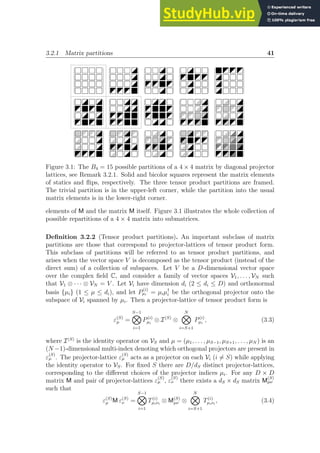
product partitions of M are illustrated by the framed images in Figure 3.1.
Remark 3.2.3 (Number of tensor product partitions). To count the number of pos-
sible tensor product partitions of a D × D matrix, we note that every factorisation
of D into k integers di ≥ 2 contributes k partitions to the total. The total number
of tensor product partitions is therefore equal to the total number of elements in all
factorisations of D. For D = 2, 3, 4, 5, 6, 7, 8, . . . this is equal to 1, 1, 3, 1, 3, 1, 6, . . .
(sequence A066637 in [52]). A special case arises when D has the form dN
, with d
prime. Then the factorisations of D into k parts are in one-to-one correspondence
with the additive partitions of N into k parts, and the number of tensor product
partitions is equal to the total number of elements in all partitions of N. For exam-
ple, matrices of dimension D = 2, 4, 8, 16, 32, . . . admit 1, 3, 6, 12, 20, . . . (sequence
A006128 in [52]) tensor product partitions.
3.2.2 The partition of matrix powers and functions
Since the matrix elements of Mk
(k ∈ N∗
= N{0}) are generated from those of
M through the rules of matrix multiplication, the partition of a matrix power can
be expressed in terms of the partition of the original matrix. Here we present this
relationship for the case of a general partition of M; the case of a tensor product
partition is identical. The proof of these results is deferred to §3.5. The partition of
Mk
is given in terms of the partition of M by Mk
ωα
=
P
ηk,...,η2
Mωηk
· · · Mη3η2 Mη2α,
where α ≡ η1, ω ≡ ηk+1, and each of the sums runs over the n values that index
the vector spaces of the general partition. It follows that the partition of a matrix
function f(M) with power series expansion f M
=
P∞
k=0 fk Mk
is
f M
ωα
=
∞
X
k=0
fk
X
ηk,...,η2
Mωηk
· · · Mη3η2 Mη2α. (3.5)
This equation provides a method of computing individual submatrices of f M
with-
out evaluating the full result. In the next section, we map the infinite sum of Eq. (3.5)
into a sum over the contributions of walks on a weighted graph, thus allowing exact
resummations of families of terms of Eq. (3.5) by applying results from graph theory.
3.2.3 The graph of a matrix partition
Given an arbitrary partition of a matrix M, we construct a weighted directed graph
G that encodes the structure of this partition. Terms that contribute to the matrix
power Mk
are then in one-to-one correspondence with walks of length k on G. The
infinite sum over walks on G involved in the evaluation of f(M) is then reduced into
a sum over simple paths on G.](https://image.slidesharecdn.com/agraphtheoreticapproachtomatrixfunctionsandquantumdynamicsphdthesis-230805203656-4458b8ad/85/A-Graph-Theoretic-Approach-To-Matrix-Functions-And-Quantum-Dynamics-PhD-Thesis-52-320.jpg)
![44 The Method of Path-Sums
(1, 0, 0, 0)T
, v2 = (0, 1, 0, 0)T
, etc. The corresponding partition of M is
M1 =
m11 m12
m21 m22
, M12 =
m13
m23
, M13 =
m14
m24
(3.7a)
M2 = m33
, M23 = m34
, M31 = m41 m42
, (3.7b)
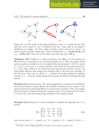
and M21 = M32 = M3 = 0. Figure 3.2 illustrates G, together with two walks of
length 4 from vertex 2 to vertex 1 that contribute to M4
12
.
The graph G provides a useful representation of a matrix partition: each ver-
tex represents a vector space in the partition, while each edge represents a linear
mapping between vector spaces. The graph G is thus a quiver and the set of vector
spaces {Vµ} together with the set of linear maps {ϕµν} is a representation of this
quiver. Further, the pattern of edges in G encodes the structure of M: each loop
(µµ) represents a non-zero static, while each link (νµ) represents a non-zero flip.
The matrix M can therefore be said to be a G-structured matrix. Every walk on
G, e.g. w = (η1)(η1η2) · · · (ηk−1ηk)(ηk), is now in one-to-one correspondence with a
product W[w] = Mηkηk−1
· · · Mη3η2 Mη2η1 of submatrices [20, 19]. This matrix product
is termed the contribution of the walk w and, being a product of matrices, is written
right-to-left. This correspondence allows a matrix power to be expressed as a sum
over contributions of walks on G. Equation (3.5) becomes
f M
ωα
=
∞
X
k=0
fk
X
WG;αω;k
W(w), (3.8)
where WG;αω;k is the set of all walks of length k from α to ω on G. We do not know
if such a formulation of f(M) would be possible for a nonprimary matrix function
and thus we only consider primary matrix functions in this thesis.
Thanks to Theorem 2.3.4 we reduce a sum of walk contributions, such as the
one of Eq. (3.8), into a sum of weighted simple paths and simple cycles. If G is a
finite graph, there is only a finite number of simple paths and simple cycles and the
resulting representation of f M
presents finitely many terms.
3.3 Path-Sum Expressions for Common Matrix
Functions
In §3.2 we showed that projector-lattices can be used to evaluate the partition of a
matrix function f M
, and further, that the resulting expression can be interpreted
as a sum over walks on a directed graph G (Eq. (3.8)). This mapping enables
results from graph theory to be applied to the evaluation of matrix power series.
In this section we exploit this connection by using Theorem 2.3.4 to resum, in
closed form, certain families of terms in the power series for the partition of some
common matrix functions. For each function we resum all terms in the power series](https://image.slidesharecdn.com/agraphtheoreticapproachtomatrixfunctionsandquantumdynamicsphdthesis-230805203656-4458b8ad/85/A-Graph-Theoretic-Approach-To-Matrix-Functions-And-Quantum-Dynamics-PhD-Thesis-54-320.jpg)
![3.3.1 A matrix raised to a complex power 45
that correspond to closed walks on G, and thereby obtain a closed-form expression
for the submatrices f(M)ωα. Since this expression takes the form of a finite sum
over simple paths on G, we refer to it as a path-sum result. The existence of a
form involving finitely many terms and giving exactly a matrix function may seem
unsurprising in view of the existence of the Cayley-Hamilton Theorem (CHT) [51].
Indeed the Theorem entails that any analytical function f of a matrix M is given
by a polynomial in M. The CHT is limited to matrices over a commutative ring
however, while the graph-theoretic origin of the path-sum result means that it is
not. As a consequence, the CHT does not have an immediate generalisation that
holds for arbitrary matrix partitions. For these reasons, if there exists a relation
between the CHT and the path-sum representation of matrix functions, it must be
that the CHT follows from the path-sum formula when all walks weights commute.
More precisely, the determinant of a matrix M has a unique expansion in terms of
simple cycles on the graph whose adjacency matrix has the same structure than
M [175]. However, this expansion, which arises from the cycle representation of
permutations, is (precisely for this reason) invariant under cyclic permutations of the
vertices visited by the simple cycles, e.g. (1231) and (2312) represent the same term.
Evidently, this holds for weighted walks if and only if all walk weights commute,
which is only true for matrices over commutative rings. This explains why there
is no block formula for the determinant and thus why the CHT fails for matrices
with non-commuting elements. One could insist on constructing a non-commutative
determinant by removing the invariance under cyclic permutations, which requires
to make the determinant entry-specific. In fact, this new object also has a path-sum
representation: it is the quasideterminant, see §3.4.5.
Below we present path-sum results for a matrix raised to a general complex
power, the matrix inverse, matrix exponential, and matrix logarithm. The results
are proved in §3.5, and examples illustrating their use are provided in §3.4.
3.3.1 A matrix raised to a complex power
Theorem 3.3.1 (Path-sum result for a matrix raised to a complex power).
Let M ∈ CD×D
be a non-nilpotent matrix, {Mµν} be an arbitrary partition of M and
q ∈ C. Then the partition of Mq
is given by
(Mq
)ωα = −Z−1
u
X
ΠG0;αω
FG{α,...,νℓ}[ω] Mωνℓ
· · · FG{α}[ν2] Mν2α FG[α]
[n]
n=−q−1
, (3.9a)
where G is the graph of {(M − I)µν}, ℓ is the length of the simple path, and
FG[α] =
Iz−1
− Mα −
X
ΓG0;α
Mαµm FG{α,...,µm−1}[µm] · · · FG{α}[µ2]Mµ2α
−1
, (3.9b)](https://image.slidesharecdn.com/agraphtheoreticapproachtomatrixfunctionsandquantumdynamicsphdthesis-230805203656-4458b8ad/85/A-Graph-Theoretic-Approach-To-Matrix-Functions-And-Quantum-Dynamics-PhD-Thesis-55-320.jpg)
![46 The Method of Path-Sums
with m the length of the simple cycle.
Here Z−1
u {g(z)} [n] denotes the inverse unilateral Z-transform of g(z) [53]. The
quantity FG[α] is defined recursively through Eq. (3.9b). Indeed FG[α] is expressed
in terms of FG{α,...,µj−1}[µj] which is in turn defined through Eq. (3.9b) but on the
subgraph G{α, . . . , µj−1} of G. The recursion stops when vertex µj has no neighbour
on this subgraph, in which case FG{α,...,µj−1}[µj] = (Iz−1
− Mµj
)−1
if the loop (µjµj)
exists and FG{α,...,µj−1}[µj] = Iz otherwise. FG[α] is thus a matrix continued fraction
which terminates at a finite depth. It is an effective weight associated to vertex α
resulting from the dressing of α by all the closed walks off α on G.
Remark 3.3.1 (Matrix pth
-roots). When analytically computing the pth
-root, p ∈
N∗
, of a matrix M using Theorem 3.3.1 one can obtain all the primary pth
-roots of
that matrix. Indeed remark first that whenever a number λ = |λ|eiθ
appears raised
to the power q = 1/p in the analytical result, one is free to choose any one of its
pth
-roots λq
|q=1/p ≡ |λ|1/p
eiθ/p
e2inπ/p
, n ∈ {0, 1, · · · , p − 1}. Second, λ is necessarily
an eigenvalue of M since, by the Jordan decomposition, Mq
= PJq
P−1
, and thus any
number raised to the power q in Mq
is one that appears on the diagonal of J. It
follows that all the primary pth
-roots of M are indeed obtained from Theorem 3.1
upon choosing different pth
-roots for the numbers λ1/p
[51].
3.3.2 The matrix inverse
Theorem 3.3.2 (Path-sum result for the matrix inverse). Let M ∈ CD×D
be
an invertible matrix, and {Mµν} be an arbitrary partition of M. Then as long as all
of the required inverses exist, the partition of M−1
is given by the path-sum
M−1
ωα
=
X
ΠG0;αω
(−1)ℓ
FG{α,...,νℓ}[ω]Mωνℓ
· · · FG{α}[ν2] Mν2α FG[α], (3.10a)
where G is the graph of {(M − I)µν}, ℓ is the length of the simple path, and
FG[α] =
Mα −
X
ΓG0;α
(−1)m
Mαµm FG{α,...,µm−1}[µm] · · · FG{α}[µ2]Mµ2α
−1
, (3.10b)
with m the length of the simple cycle.
If α has no neighbours in G then FG[α] = M−1
α counts the contributions of all loops
on α.
Remark 3.3.2 (Known inversion formulae). Two known matrix inversion results
can be straightforwardly recovered as special cases of Theorem 3.3.2. Firstly, by
considering the complete directed graph on two vertices, we obtain the well-known
block inversion formula
A B
C D
−1
=
(A − BD−1
C)
−1
−A−1
B (D − CA−1
B)
−1
−D−1
C (A − BD−1
C)
−1
(D − CA−1
B)
−1
. (3.11)](https://image.slidesharecdn.com/agraphtheoreticapproachtomatrixfunctionsandquantumdynamicsphdthesis-230805203656-4458b8ad/85/A-Graph-Theoretic-Approach-To-Matrix-Functions-And-Quantum-Dynamics-PhD-Thesis-56-320.jpg)
![3.3.3 The matrix exponential 47
Secondly, by applying Theorem 3.3.2 to the path-graph on N ≤ D vertices (denoted
here PN ), we obtain known continued fraction formulae for the inverse of a D × D
block tridiagonal matrix [54, 55, 56, 57]. This follows from the observation that a
PN -structured matrix is a block tridiagonal matrix. We provide a general formula
for the exponential and inverse of arbitrary PN -structured matrices in §3.4.3.
Remark 3.3.3 (Path-sum results via the Cauchy integral formula). A path-sum
expression can be derived for any matrix function upon using Theorem 3.3.2 together
with the Cauchy integral formula
f(M) =
1
2πi
I
Γ
f(z) (zI − M)−1
dz, (3.12)
where i2
= −1, f is an holomorphic function on an open subset U of C and Γ
is a closed contour completely contained in U that encloses the eigenvalues of M.
However, for certain matrix functions (including all four we consider in this section)
a path-sum expression can be derived independently of the Cauchy integral formula
by using Theorem 2.3.4 directly on the power series for the function. This method
is the one we use to prove the results of this section (see §3.5) and can be extended
to matrices over division rings.
Remark 3.3.4 (Schur decomposition). Let M ∈ CD×D
, M = UTU−1
be its Schur
decomposition, i.e. T is upper triangular, and let {Mµν} a partition of M. The
difficulty of evaluating f(M) if M is full can be alleviated upon using the Schur
decomposition of M in conjunction with the method of path-sums. Indeed observe
that
f(M)
ωα
=
X
µ, ν
Uωµ f(T)
µν
(Uαν)†
, (3.13)
where we have used U−1
= U†
and (U†
)να = (Uαν)†
. Thus the problem of evaluating
any (f(M))ωα is reduced to that of evaluating f(T). Now remark that regardless of
the partition {Tµν} considered, the graph G of that partition has no simple cycle
of length m 1. Thus the path-sum formula for any matrix function f(T) is
especially simple. For example consider obtaining f(T) via the Cauchy integral
formula Eq. (3.12). Then the resolvent matrix RT(z) = (zI − T)−1
of T is given by
the path-sum
RT(z)
µν
=
X
ΠG0;νµ
(zI − Tµ)−1
Mµηℓ
· · · Mη2ν (zI − Tν)−1
, (3.14a)
RT(z)
µ
= (zI − Tµ)−1
, (3.14b)
where G is the graph of {Tµν} and ℓ is the length of the simple path.
3.3.3 The matrix exponential](https://image.slidesharecdn.com/agraphtheoreticapproachtomatrixfunctionsandquantumdynamicsphdthesis-230805203656-4458b8ad/85/A-Graph-Theoretic-Approach-To-Matrix-Functions-And-Quantum-Dynamics-PhD-Thesis-57-320.jpg)
![48 The Method of Path-Sums
Theorem 3.3.3 (Path-sum result for the matrix exponential). Let M ∈ CD×D
and {Mµν} be an arbitrary partition of M, with G the corresponding graph. Then for
τ ∈ C the partition of exp(τM) is given by the path-sum
exp(τM)ωα = L−1
X
ΠG0;αω
FG{α,...,νℓ}[ω]Mωνℓ
· · · FG{α}[ν2] Mν2α FG[α]
(t)
t =τ
,(3.15a)
where ℓ is the length of the simple path and
FG[α] =
sI − Mα −
X
ΓG0;α
Mαµm FG{α,...,µm−1}[µm] · · · FG{α}[µ2]Mµ2α
−1
, (3.15b)
with m the length of the simple cycle.
Here s is the Laplace variable conjugate to t, and L−1
{g(s)}(t) denotes the inverse
Laplace transform of g(s). The quantity FG[α] is a matrix continued fraction which
terminates at a finite depth. It is an effective weight associated to vertex α resulting
from the dressing of α by all the closed walks off α on G. If α has no neighbours in
G then FG[α] = [sI − Mα]−1
counts the contributions of all loops off α.
Lemma 3.3.1 (Walk-sum result for the matrix exponential). Let M ∈ CD×D
and
{Mµν} be an arbitrary partition of M, with G the corresponding graph. Then for
τ ∈ C the partition of exp(τM) is given by the walk-sum
exp(τM)ωα =
X
WG0;αω
Z τ
0
dtm · · ·
Z t2
0
dt1 exp
(t − tm)Mω
Mωµm · · ·
· · · exp
(t2 − t1)Mµ2
Mµ2α exp
t1Mα
. (3.16)
This result corresponds to dressing the vertices only by loops, instead of by all closed
walks. An infinite sum over all walks from α to ω on the loopless graph G0 therefore
remains to be carried out.
3.3.4 The matrix logarithm
Theorem 3.3.4 (Path-sum result for the principal logarithm). Let M ∈
CD×D
be a matrix with no eigenvalues on the negative real axis, and {Mµν} be a
partition of M. Then as long as all of the required inverses exist, the partition of the](https://image.slidesharecdn.com/agraphtheoreticapproachtomatrixfunctionsandquantumdynamicsphdthesis-230805203656-4458b8ad/85/A-Graph-Theoretic-Approach-To-Matrix-Functions-And-Quantum-Dynamics-PhD-Thesis-58-320.jpg)
![3.4. Applications 49
principal matrix logarithm of M is given by the path-sum
log M
ωα
= (3.17a)
Z 1
0
dx x−1
(I − FG[α]) , ω = α,
X
ΠG0;αω
Z 1
0
dx (−x)ℓ−1
FG{α,...,νℓ}[ω]Mωνℓ
· · · FG{α}[ν2] Mν2α FG[α], ω 6= α,
where G is the graph of {(I − M)µν}, ℓ the length of the simple path and
FG[α] = (3.17b)
I − x(I − Mα) −
X
ΓG0;α
(−x)m
Mαµm FG{α,...,µm−1}[µm] · · · Mµ3µ2 FG{α}[µ2]Mµ2α
−1
,
with m the length of the simple cycle.
The quantity FG[α] is a matrix continued fraction which terminates at a finite depth.
It is an effective weight associated to vertex α resulting from the dressing of α
by all the closed walks off α on G. If α has no neighbours in G then FG[α] =
[I − x(I − Mα)]−1
counts the contributions of all loops off α.
Remark 3.3.5 (Richter relation). The path-sum expression of Theorem 3.3.4 is
essentially the well-known integral relation for the matrix logarithm [58, 59, 51]
log M =
Z 1
0
(M − I)
x(M − I) + I
−1
dx, (3.18)
with a path-sum expression of the integrand. However, the proof of Theorem 3.3.4
that we present in 3.5.5 does not make explicit use of Eq. (3.18).
3.4 Applications
In this section we present some examples of the application of the path-sum method.
In the first part we provide numerical examples for a matrix raised to a complex
power, the matrix inverse, exponential, and logarithm. In the second part, we
provide exact results for the matrix exponential and matrix inverse of block tridi-
agonal matrices and evaluate the computational cost of path-sum on arbitrary tree-
structured matrices.
3.4.1 Short examples
Example 3.4.1 (Singular and defective matrix raised to an arbitrary complex
power). To illustrate the result of Theorem 3.3.1, we consider raising the matrix](https://image.slidesharecdn.com/agraphtheoreticapproachtomatrixfunctionsandquantumdynamicsphdthesis-230805203656-4458b8ad/85/A-Graph-Theoretic-Approach-To-Matrix-Functions-And-Quantum-Dynamics-PhD-Thesis-59-320.jpg)
![50 The Method of Path-Sums
M =
−4 0 −1 0 −1
−2 −2 6 −2 4
6 2 1 −2 3
0 0 −1 −4 −1
−6 −2 −5 2 −7
, (3.19)
to an arbitrary complex power q. Note that M has a spectral radius ρ(M) = 4 and
is both singular and defective; i.e. non-diagonalisable. We partition M onto vector
space V1 = span v1, v2
and V2 = span v3, v4, v5
with v1 = (1, 0, 0, 0)T
etc., such
that V1 ⊕V2 = V . The corresponding graph G is the complete graph on two vertices,
denoted K2. Following Theorem 3.3.1, the elements of Mq
are given by,
(Mq
)ii = −Z−1
u
FK2 [i] [n]
n=−q−1
and (Mq
)ij = −Z−1
u
FK2j[i]M12FK2 [j] [n]
n=−q−1
, (3.20)
where (i, j) = 1, 2, i 6= j, FK2 [i] =
Iz−1
− Mi − MijFK2i[j]Mji
−1
and FK2i[j] =
[Iz−1
− Mj]
−1
. We thus find in the Z-domain
M̃(z) = z(4z + 1)−2
× (3.21)
4z + 1 0 −z 0 −z
2z(4z − 1) 8z2
+ 6z + 1 88z3+50z2+6z
4z+1
−2z(4z + 1) 56z3+34z2+4z
4z+1
2z(4z + 3) 2z(4z + 1) 88z3+54z2+13z+1
4z+1
−2z(4z + 1) 56z3+22z2+3z
4z+1
0 0 −z 4z + 1 −z
−2z(4z + 3) −2z(4z + 1) −88z3+38z2+5z
4z+1
2z(4z + 1) −56z3−6z2+5z+1
4z+1
.
and finally Mq
= −Z−1
u {M̃(z)}[n]|n=−q−1, which is
Mq
=
(−4)q
8
8 0 2q 0 2q
8q − 4 4 q(q − 2) − 11 4 q(q − 2) − 7
−8q − 4 −4 −q(q − 2) − 3 4 −q(q − 2) − 7
0 0 2q 8 2q
8q + 4 4 q(q − 2) + 11 −4 q(q − 2) + 15
. (3.22)
This expression is valid for any q ∈ C and fulfills Mq+q′
= Mq
Mq′
, ∀(q, q′
) ∈ C2
.
Setting q = 1/2, we obtain
M1/2
=
i
16
32 0 4 0 4
0 16 −47 16 −31
−32 −16 −9 16 −25
0 0 4 32 4
32 16 41 −16 57
, (3.23)](https://image.slidesharecdn.com/agraphtheoreticapproachtomatrixfunctionsandquantumdynamicsphdthesis-230805203656-4458b8ad/85/A-Graph-Theoretic-Approach-To-Matrix-Functions-And-Quantum-Dynamics-PhD-Thesis-60-320.jpg)
![3.4.1 Short examples 51
with i2
= −1, for which it is easily verified that (M1/2
)2
= M. Any pth
root of M,
with p ∈ N∗
, can also be calculated and verified. Further, we note that although M
is not invertible, setting q = −1 in Eq. (3.22) yields the Drazin inverse M♯
of M [60],
while setting q = 0 yields a left and right identity M♭
on M
M♯
=
1
16
−4 0 1 0 1
6 −2 4 −2 2
−2 2 3 −2 5
0 0 1 −4 1
2 −2 −7 2 −9
, M♭
=
1
8
8 0 0 0 0
−4 4 −11 4 −7
−4 −4 −3 4 −7
0 0 0 8 0
4 4 11 −4 15
.
(3.24)
The above Drazin inverse satisfies indeed MM♯
M = M, M♯
MM♯
= M♯
and M♯
Mq
=
Mq
M♯
= Mq−1
. We also have M: M♭
Mq
= Mq
M♭
= Mq
for any q ∈ C and finally
M♯
M = MM♯
= M♭
as expected of the Drazin inverse. These properties imply that
M♭
is the projector onto im(M), the image of M. We demonstrate in §3.4.2 that
Theorem 3.3.1 always produces the Drazin inverse.
In addition to the examples with q = −1, 0, and 1/p with p ∈ N∗
presented here,
the formula of Eq. (3.22) also holds for any complex value of q and is well behaved.
For example, we verify analytically using Theorem 3.3.1 to calculate (M±i
)q
that
(M±i
)∓i
= M. Finally, it is noteworthy that numerical methods implemented by
standard softwares such as MATLAB and Mathematica suffer from serious stability
problems for the matrix considered here and return incorrect results, as can be seen
for the case of q = 1/2.
Example 3.4.2 (Matrix inverse). To illustrate the application of Theorem 3.3.2 we
compute the inverse of
M =
−1 0 0 0 −1/2
0 2 5/2 2 −1
−4 0 0 0 −1
0 −1 0 −2 7/4
0 1 2 0 1
. (3.25)
The characteristic polynomial of M is χ(x) = x5
− x − 1, whose Galois group is
the symmetric group S5 and is thus non-solvable. The spectral radius of M is
ρ(M) ≃ 1.16. We partition M onto vector spaces V1 = span v1
, V2 = span v3, v5
and V3 = span v2, v4
, giving
M1 = −1
, M2 =
0 −1
2 1
, M3 =
2 2
−1 −2
, (3.26)
M12 = 0 −1/2
, M21 =
−4
0
, M23 =
0 0
1 0
, M32 =
5/2 −1
0 7/4
, (3.27)
and M13 = M31 = 0. The corresponding graph is thus the path-graph on three
vertices, denoted by P3. By Theorem 3.3.2, the diagonal elements of M−1
are given](https://image.slidesharecdn.com/agraphtheoreticapproachtomatrixfunctionsandquantumdynamicsphdthesis-230805203656-4458b8ad/85/A-Graph-Theoretic-Approach-To-Matrix-Functions-And-Quantum-Dynamics-PhD-Thesis-61-320.jpg)
![52 The Method of Path-Sums
by
M−1
11
= FL3 [1], M−1
22
= FL3 [2], M−1
33
= FL3 [3], (3.28a)
while the off-diagonal elements are
M−1
21
= −FL3{1}[2] M21 FL3 [1], M−1
12
= −FL3{2}[1] M12 FL3 [2], (3.28b)
M−1
32
= −FL3{2}[3] M32 FL3 [2], M−1
23
= −FL3{3}[2] M23 FL3 [3], (3.28c)
M−1
31
= FL3{1,2}[3] M32 FL3{1}[2] M21 FL3 [1], (3.28d)
M−1
13
= FL3{3,2}[1] M12 FL3{3}[2] M23 FL3 [3]. (3.28e)
The matrices FG[α] are evaluated according to the recursive definition in Eq. (3.10b);
for example
FL3 [1] =
M1 − M12FL3{1}[2]M21
−1
=
M1 − M12[M2 − M23FL3{1,2}[3]M32]−1
M21
−1
,
=
M1 − M12[M2 − M23M−1
3 M32]−1
M21
−1
. (3.29)
Evaluating the flips and statics and reassembling them into matrix form gives
M−1
=
1
8
8 0 −4 0 0
64 −32 −16 −32 40
−16 16 4 16 −16
−60 16 15 12 −20
−32 0 8 0 0
, (3.30)
which is readily verified to be the inverse of M.
Example 3.4.3 (Matrix exponential). As an example of the application of Theorem
3.3.3 and Lemma 3.3.1 we consider the matrix exponential of
M =
1 − i 0 −i 0
0 2 − i −1/3 0
i 0 −i 0
3 −7/2 1 −1
. (3.31)
We use a tensor product partition
M1 =
1 − i 0
0 2 − i
, M2 =
−i 0
1 −1
, M12 =
−i 0
−1/3 0
, M21 =
i 0
3 −7/2
.
Since every element of this matrix partition is non-zero, the corresponding graph is
K2. Let us focus on the element exp(M)11, which forms the top-left corner of the](https://image.slidesharecdn.com/agraphtheoreticapproachtomatrixfunctionsandquantumdynamicsphdthesis-230805203656-4458b8ad/85/A-Graph-Theoretic-Approach-To-Matrix-Functions-And-Quantum-Dynamics-PhD-Thesis-62-320.jpg)
![3.4.1 Short examples 53
full matrix exp(M). By Theorem 3.3.3 the exact result for exp(tM)11 is given by
L
etM
11
= FK2 [1] =
sI − M1 − M12[sI − M2]−1
M21
−1
, (3.32a)
=
s + i
s2 − (1 − 2i)s − (2 + i)
0
−i
3s3 − (9 − 9i)s2 − (6 + 18i)s + 15
1
s − (2 − i)
.
(3.32b)
The inverse Laplace transform can be carried out analytically; setting t = 1 in the
result gives
eM
11
=
e(1−2i)/2
15
3
5 cosh
√
5
2
+
√
5 sinh
√
5
2
0
−i
5e3/2
− 5 cosh
√
5
2
− 3
√
5 sinh
√
5
2
15 e3/2
, (3.33a)
≈
2.05220 − 3.19611 i 0
−0.442190 − 0.283927 i 3.99232 − 6.21768 i
. (3.33b)
Alternatively, we can evaluate this element by using a walk-sum, as presented in
Lemma 3.3.1:
eM
11
= eM1
+
Z 1
0
Z t2
0
e(1−t2)M1
M12 e(t2−t1)M2
M21 et1M1
dt1 dt2 (3.34)
+
Z 1
0
· · ·
Z t2
0
e(1−t4)M1
M12 e(t4−t3)M2
M21 e(t3−t2)M1
M12 e(t2−t1)M2
M21 et1M1
dt1 · · · dt4 + · · ·
Evaluating the first three terms yields
eM
11
≃
2.05083 − 3.19398 i 0
−0.441354 − 0.283390 i 3.99232 − 6.21768 i
. (3.35)
Although this result has been obtained by evaluating only the first three terms
of an infinite series, it is already an excellent approximation to the exact answer:
the maximum absolute elementwise error is ∼ 2.5 × 10⁻³
. This rapid convergence
results from the exact resummation of the terms in the original Taylor series that
correspond to walks on the graph K2 that contain loops.
Example 3.4.4 (Matrix logarithm of a defective matrix). We compute the principal
logarithm of the matrix
M =
−1 + 2i −1 + 2i 1 2 − 2i −2 + 2i
−1 −1 + 2i 1 − 2i 1 −2 + 2i
0 1 2i 0 1
−1 −1 + 2i 1 2 −2 + 2i
0 1 −1 + 2i 0 2
. (3.36)](https://image.slidesharecdn.com/agraphtheoreticapproachtomatrixfunctionsandquantumdynamicsphdthesis-230805203656-4458b8ad/85/A-Graph-Theoretic-Approach-To-Matrix-Functions-And-Quantum-Dynamics-PhD-Thesis-63-320.jpg)
![54 The Method of Path-Sums
This matrix has only two eigenvectors associated respectively to the three-fold de-
generate eigenvalue 2i and to the two-fold degenerate eigenvalue 1. We choose to par-
tition M onto vector spaces V1 = span v1, v4
, V2 = span v2, v3
and V3 = span v5
.
The corresponding graph G is the complete directed graph on three vertices with
the edge (13) missing since M31 = 0 0
. Following Theorem 3.3.4 we have
FG[1] =
I1 − x(I1 − M1) − x2
M12FG1[2]M21 + x3
M13FG1,2[3]M32FG1[2]M21
−1
, (3.37a)
FG[3] =
I3 − x(I3 − M3) − x2
M32FG3[2]M23 + x3
M32FG1,3[2]M21FG3[1]M13
−1
, (3.37b)
FG[2] =
I2 − x(I2 − M2) − x2
M21FG2[1]M12 − x2
M23FG2[3]M32
+ x3
M21FG2,3[1]M13FG2[3]M32
−1
, (3.37c)
with Ii the identity matrix of appropriate dimension and
FGi[j] =
I − x(I − Mj) − x2
MjkFGi,j[k]Mkj
−1
, i 6= 2, (3.38a)
FG2[j] = FGi,k[j] =
I − x(I − Mj)
−1
. (3.38b)
with i, j, k = (1, 2, 3), i 6= j 6= k. Then the matrix elements of the principal
logarithm of M are given by
log M
ii
=
Z 1
0
x−1
(I − FG[i]) dx, (3.39a)
log M
31
=
Z 1
0
−x FG1,2[3]M32FG1[2]M21FG[1] dx, (3.39b)
log M
ji
=
Z 1
0
FGi[j]MjiFG[i] dx, i, j = (1, 2) or (2, 3) (3.39c)
and for i, j = (2, 1), (3, 1) or (3, 2):
log M
ji
=
Z 1
0
FGi[j]MjiFG[i] − x FGi,k[j]MjkFGi[k]MkiFG[i] dx. (3.39d)
Reassembling them in a matrix, we obtain
log M =
1
2
λ + i λ 2 −λ − i λ − 2
1
4
+ i λ + i −λ −1
4
− i λ + i
−1
4
−i λ 1
4
−i
i λ 2 −i λ − 2
−1
4
−i λ 1
4
−i
, (3.40)
where λ = 2 log 2 + iπ.
Example 3.4.5 (Matrix exponential of a quaternionic matrix). Consider any func-
tion f(z) =
P
n anzn
with an ∈ R for all n ∈ N. Then the graph-theoretic nature of
Theorem 2.3.4 allows the method of path-sums to be extended to matrices over non-
commutative division rings D. In particular, Theorems 3.3.1-3.3.4 hold for quater-
nionic matrices M ∈ HD×D
as well. For example, consider calculating exp(πM) with](https://image.slidesharecdn.com/agraphtheoreticapproachtomatrixfunctionsandquantumdynamicsphdthesis-230805203656-4458b8ad/85/A-Graph-Theoretic-Approach-To-Matrix-Functions-And-Quantum-Dynamics-PhD-Thesis-64-320.jpg)
![3.4.2 Generalised matrix powers 55
M the quaternionic matrix
M =
i j
k 1
, (3.41)
where i, j, and k are the quaternions, which satisfy i2
= j2
= k2
= i j k = −1.
Following Theorem 3.3.3, we find for example the matrix element M11 to be in the
Laplace domain
L
exp(tM)11
= (s − i − j(s − 1)−1
k)−1
. (3.42)
Calculating the other matrix elements, inverting the Laplace transforms and setting
t = π, we obtain
exp(πM) = −
1 + eπ
2
i + tanh π
2
j − k
k − j i + tanh π
2
. (3.43)
3.4.2 Generalised matrix powers
The matrix roots are among the most studied matrix functions [51] with numerous
applications from finance to healthcare [61]. It is well known that a matrix may fail
to have a pth
-root [51]. For example, a matrix M has a square root, defined by the
relation
√
M
2
= M, if and only if the ascent sequence d1, d2 · · · defined by
di = dim ker(Mi
)
− dim ker(Mi−1
)
, (3.44)
does not comprise the same odd integer twice or more [62]. Just as a matrix may
fail to have a square root, it can fail to have an inverse, yet it always has generalised
inverses. Similarly, we show in this section that a matrix always has generalised
powers, which we obtain with the method of path-sums.
Definition 3.4.1 (Generalised matrix powers). Let M ∈ CD×D
and let M|ker(M) and
M|im(M) be the restrictions of M to its kernel and image, respectively. Then the
generalised powers of M are defined as
Mq
gen = M|im(M)
q
. (3.45)
We will see that the Drazin inverse of M is recovered as the generalised power M−1
gen
and thus also call Mq
gen the Drazin powers of M. We obtain the generalised matrix
powers using the method of path-sums as follows:
Proposition 3.4.1. Let M̃(z) be the matrix defined by the path-sums on the right
hand side of Eqs. (3.9a, 3.9b). Then the ordinary powers Mq
ord = M|ker(M)
q
+
M|im(M)
q
and generalised powers Mq
gen = M|im(M)
q
of M are given by
Mq
ord = −Z−1
b
M̃(z) [n]
n=−q−1
, Mq
gen = −Z−1
u
M̃(z) [n]
n=−q−1
. (3.46)
Here Z−1
b {.}[n] and Z−1
u [.] denote respectively the bilateral and unilateral inverse
Z-transforms.](https://image.slidesharecdn.com/agraphtheoreticapproachtomatrixfunctionsandquantumdynamicsphdthesis-230805203656-4458b8ad/85/A-Graph-Theoretic-Approach-To-Matrix-Functions-And-Quantum-Dynamics-PhD-Thesis-65-320.jpg)
![56 The Method of Path-Sums
Proof. Let M ∈ CD×D
with dim(ker(M)) = k0 and non-zero eigenvalues {λl}1≤l≤D−k0 .
Consider the matrix M̃(z) obtained in the Z-domain by the path-sum formula, The-
orem 3.3.1. Let M = PJP−1
be the Jordan decomposition of M. Observe that since
Mq
= PJq
P−1
, M̃(z) = P[z−1
− J]−1
P−1
and the entries of M̃(z) are of the form
M̃(z)
ij
=
Qij(z) zk0
QD−k0
l=1 (λl − z−1)
, (3.47)
with Qij(z) a polynomial in z. A partial fraction decomposition of the matrix entries
separate terms with exclusively positive powers of z from those involving fractions
of z. Thus, we can write
M̃(z)
ij
=
D−1
X
p=1
αpzp
+
Pij(z)
QD−k0
l=1 (λlz − 1)
, (3.48)
where Pij(z) is a polynomial in z and αp ∈ C are the coefficients of the decom-
position. Terms with strictly positive powers of z arise because of the zk0
factor
in Eq. (3.47) and thus correspond to the kernel of the matrix. These terms are
discarded by the unilateral inverse Z-transform, and
Mq
gen
ij
= −Z−1
u
n Pij(z)
QD−k0
l=1 (λlz − 1)
)
o
[n]
n=−q−1
, (3.49)
represents M|im(M)
q
, the powers of M restricted to its image. On the contrary,
a bilateral inverse Z-transform conserves the terms associated with the kernel and
yields ordinary powers
Mq
ord
ij
= −Z−1
b
n Qij(z) zk0
QD−k0
l=1 (λl − z−1)
o
[n]
n=−q−1
. (3.50)
The two agree when M is not singular. Finally, remark that since M−1
gen = M|im(M)
−1
we have M−1
gen = M♯
as claimed.
The method of path-sums, in conjunction with the appropriate inverse Z-transform,
gives generalised as well as ordinary powers of a matrix. The generalised matrix pow-
ers always exist. We call them Drazin powers because they share the properties of
the Drazin inverse: they coincide with the ordinary powers for non-singular matrices
and [Mq
, M] = 0, Mq
Mq′
= Mq+q′
, M−1
= M♯
, M0
= M♭
= M♯
M, M1/2
M1/2
= M♭
etc.
All of these properties are straightforward consequences of Mq
gen = M|im(M)
q
.
Example 3.4.6 (Generalised and ordinary powers of a singular defective matrix).](https://image.slidesharecdn.com/agraphtheoreticapproachtomatrixfunctionsandquantumdynamicsphdthesis-230805203656-4458b8ad/85/A-Graph-Theoretic-Approach-To-Matrix-Functions-And-Quantum-Dynamics-PhD-Thesis-66-320.jpg)
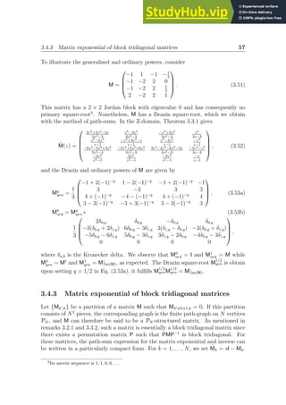
![58 The Method of Path-Sums
and define the finite continued fractions
X̃k =
h
M̃k − Mk,k+1X̃k+1Mk+1,k
i−1
, Ỹk =
h
M̃k − Mk,k−1Ỹk−1Mk−1,k
i−1
, (3.54)
with X̃N ≡ M̃−1
N and Ỹ1 ≡ M̃−1
1 . Note that the inversion height of X̃k (Ỹk) is N +1−k
(k). Let Ũ = L[exp(t M)] be the Laplace transform of the matrix exponential of M;
then the partition of Ũ is given by
Ũkk =
h
X̃−1
k + Ỹ−1
k − M̃k
i−1
, (3.55a)
Ũk,k′k =
k
Y
j=k′+1
X̃jMj,j−1
Ũk′k′ , Ũk,k′k =
k
Y
j=k′−1
ỸjMj,j+1
Ũk′k′ , (3.55b)
where
Qn
j=1 aj = anan−1 · · · a2a1 is a left product. Provided the required inverse
Laplace-transforms are analytically available, Eq.(3.54-3.55b) yields the exact ma-
trix exponential of M. Similar formulae for the inverse of arbitrary PN -structured
matrices are obtained upon replacing sI by I in each of the M̃k.
3.4.4 Computational cost on tree-structured matrices
The number of simple paths in any finite graph is finite. Thus, as soon as a matrix
M has a finite size, the path-sum expressions of Theorems 3.3.1-3.3.4 evaluate any
function f(M) exactly in a finite number ρ of operations, up to the integral trans-
forms. In this final example we calculate ρ in the case of matrices M whose partition
is an arbitrary tree, denoted by TN .
First, we consider the computational cost of evaluating a static f(M)αα. Since a
tree contains no simple cycles of length greater than 2, the vertex α requires dressing
only by loops and edge cycles on TN . Consequently, the sequence of operations
involved in dressing α fall into two categories: nesting (adding an edge cycle which
dresses the internal vertex of a previous edge cycle) or branching (including an
extra edge cycle at constant dressing depth). These two operations have the same
computational cost, as each requires one inversion, two multiplications and one
subtraction of d×d matrices. Due to this symmetry between branching and nesting,
the computational costs of dressing a vertex on the path-graph on N vertices PN
(which involves nesting only) and the star graph on N vertices SN (which involves
branching only) are identical: each requires N inversions, 2(N − 1) multiplications
and N − 1 additions to fully dress any vertex. Since any tree can be decomposed as
a set of path-graphs (the branches) and star graphs (the nodes), the computational
cost of evaluating f(M)αα when M is tree-structured depends only on the number
of vertices of the tree: the cost is independent of the detailed structure of TN .
The number of floating point operations required to evaluate the diagonal element
f(M)αα, denoted by ρTN ;α, scales as 3Nd3
, while the computational density (the
number of operations per usual matrix-element evaluated) is ∼ 3Nd.
We now consider the cost of calculating an off-diagonal element f(M)ωα. Let](https://image.slidesharecdn.com/agraphtheoreticapproachtomatrixfunctionsandquantumdynamicsphdthesis-230805203656-4458b8ad/85/A-Graph-Theoretic-Approach-To-Matrix-Functions-And-Quantum-Dynamics-PhD-Thesis-68-320.jpg)
![3.4.5 Quasideterminants 59
(αν2 · · · νℓω) be the unique simple path leading from α to ω on TN , and ρTN ;α be the
cost of fully dressing the vertex α on TN . Then the total cost of evaluating f(M)ωα
is
2ℓd3
+
ℓ+1
X
i=1
ρTN {α,...,νi−1};νi
, (3.56)
where the first term accounts for the cost of evaluating the matrix multiplications
along the simple path. Note that this cost depends on the structure of TN , since
the number of vertices in each tree in the sequence TN {α, . . . , νi−1} depends on
whether any of the previously-visited vertices are nodes of TN . Nevertheless, we can
place an upper bound on the cost by considering the case where the tree TN is the
path-graph PN . Then PN {α, . . . , νi−1} contains N + 1 − i vertices, and the total
cost of evaluating the contribution of a simple path of length ℓ is ∼ ℓd3
(3N + 2).
Finally, we note that in the course of evaluating the contribution of a certain simple
path p, we simultaneously evaluate the contributions of all subpaths of p. The
operations counted by Eq. (3.56) therefore generate (ℓ+1)d2
elements of the partition
of f M
. This improves the computational density of the path-sum method for tree-
structured matrices to ∼ 3Nd. Therefore, we conclude that evaluating any element
of a partition of a matrix function of a tree-structured matrix using path-sums is
efficient: i.e. the cost is linear in the number of vertices in the tree.
3.4.5 Quasideterminants
The determinant is a concept of central importance in commutative linear algebra.
Initially, interest in the determinant lay in its equation-solving properties. Similarly,
noncommutative analogues to the determinants were investigated in the context of
systems of equations involving quaternions from the end of 19th
century onwards[63,
64]. The concept of quasideterminant first arose in the late 1920s [65, 66, 67]. More
recently, research on quasideterminants was revived by a series of papers by Gel’fand
and coworkers [68, 69, 70] who discovered that they share some equation solving
properties of the usual determinant, see [36]. Consequently, quasideterminants found
many applications in mathematics [71, 72, 73, 74] and mathematical-physics [75, 76,
77, 78]. We begin by defining the quasideterminants following [36].
Definition 3.4.2 (Quasideterminants [36]). Let X be a D × D matrix with formal
entries xij. Then X is invertible over the free division ring D(X) generated by
X = {xij}1≤i≤D,1≤j≤D and let Y = X−1
= (yij). The (i, j)th quasideterminant of X
is the element of D(X) defined by
|X|ij = (yji)−1
. (3.57)
The quasideterminants are therefore inverses of the elements of the transpose of
the matrix inverse of a matrix over a division ring. The reason for this seemingly
complicated definition is that quasideterminants obey a simple heredity principle.](https://image.slidesharecdn.com/agraphtheoreticapproachtomatrixfunctionsandquantumdynamicsphdthesis-230805203656-4458b8ad/85/A-Graph-Theoretic-Approach-To-Matrix-Functions-And-Quantum-Dynamics-PhD-Thesis-69-320.jpg)
![60 The Method of Path-Sums
Proposition 3.4.2 (Heredity principle [36]). Let X ∈ DD×D
. If D = 1, then
|X|11 = x11. Otherwise, for D ≥ 2, let Xij
be the (D − 1) × (D − 1) matrix obtained
from X upon deleting row the ith row and jth column. Then
|X|ij = xij − rj
i |Xij
|−1•
ci
j, (3.58)
where M−1•
designates the entry-wise (Hadamard) inverse of M, rj
i ∈ D1×(D−1)
and
ci
j ∈ D(D−1)×1
are respectively the ith row and the jth column of X with xij removed.
As we shall see, the heredity principle above is recovered by the path-sum result
in the case of the K2 graph4
. We begin with a definition necessary to state the
path-sum result on quasideterminants in full generality.
Definition 3.4.3 (Quasideterminantal matrices). Let X ∈ DD×D
and {|X|ωα} be a
partition of X. The elements |X|ωα of this partition are called quasideterminantal
matrices.
Theorem 3.4.1 (Generalised heredity principle for quasideterminantal ma-
trices). Consider X ∈ DD×D
, let Xαω be a general partition of X and let G be the
graph of {I − X}αω. Then, as long as all of the required inverses exist, the quaside-
terminantal matrices X ωα
are given by the path-sum
X
−1•
ωα
=
X
ΠG; αω
(−1)ℓp
X(α, ... , νℓp )
−1
ωω
Xωνℓp
· · · X(α)
−1
ν2
Xν2α X−1
α , (3.59a)
where ℓp is the length of the simple path and
X
−1•
α
=
h
Xα −
X
ΓG0; α
(−1)ℓc
Xαµℓc
X(α, ... , µℓc−1)
−1
µℓc µℓc
· · · X(α)
−1
µ2µ2
Xµ2α
i−1
, (3.59b)
with ℓc the length of the bare cycle. In these expressions M−1•
designates the entry-
wise inverse of M.
Proof. We start with Proposition 1.2.8 of [36], where the authors remark that
quasideterminants can be written as a sum of weighted walks on a weighted di-
graph5
. With our notation, their result reads
|I − X|ii = 1 −
X
w∈WG; ii
W[w], |I − X|−1
ij =
X
w∈WG; ji
W[w]. (3.60)
This is just the representation of the power-series for the matrix inverse as a walk
series (see more generally Eq. (3.5) of §3.2.2) in the case where the matrix is par-
titioned into its usual matrix elements. This extends straightforwardly to general
4
Complete graph on 2 vertices.
5
The authors use the term path for our walk, simple path from i to i for our cycle off vertex i,
and word to designate the weight of a walk.](https://image.slidesharecdn.com/agraphtheoreticapproachtomatrixfunctionsandquantumdynamicsphdthesis-230805203656-4458b8ad/85/A-Graph-Theoretic-Approach-To-Matrix-Functions-And-Quantum-Dynamics-PhD-Thesis-70-320.jpg)
![3.5. Proofs of Path-Sum Expressions for Common Matrix Functions 61
partitions
|I − X|αα = 1 −
X
w∈WG; αα
W[w], |I − X|−1
αω =
X
w∈WG; ωα
W[w], (3.61)
and the generalised heredity principle for quasideterminantal matrices follows di-
rectly from the weighted path-sum Theorem 2.3.4.
Remark 3.4.1 (Standard heredity principle). The standard heredity principle for
the quasideterminants of a matrix with formal entries follows directly from Theorem
3.4.1 in the case where X is partitioned onto K2, the complete undirected graph
on two vertices. To see this, let P be a permutation matrix such that xij is a
diagonal element of (PXPT
). The partition of PXPT
into four blocks PXPT
α
≡ xij,
PXPT
ω
≡ Xij
and thus Xωα ≡ ci
j, Xαω ≡ rj
i is a valid general partition of PXPT
and hence of X. Then Eq. (3.59b) reads
|X|−1•
α =
Xα − Xαω X−1
ω Xωα
−1
=⇒ |X|ij = xij − rj
i |Xij
|−1•
ci
j , (3.62)
which is the standard heredity principle.
3.5 Proofs of Path-Sum Expressions for Common
Matrix Functions
In this section we prove the path-sum results presented earlier without proof. We
begin by proving the results of §3.2.2 relating the partitions of Mk
and f(M) to the
partition of M. We then prove the path-sum results for a matrix raised to a complex
power (§3.5.2), the matrix inverse (§3.5.3), the matrix exponential (§3.5.4), and the
matrix logarithm (§3.5.5).
3.5.1 Partitions of matrix powers and functions
Consider an element RωMk
RT
α of a general partition of Mk
. On inserting the identity
in the form of the closure relation over projector-lattices between each appearance
of M in the product and using εµ = RT
µ Rµ, we obtain [20, 19]
Mk
ωα
=
X
ηk,...,η2
RωM RT
ηk
Rηk
· · · M RT
η2
Rη2 M RT
α =
X
ηk,...,η2
Mωηk
· · · Mη3η2 Mη2α, (3.63)
with α ≡ η1 and ω ≡ ηk+1. This expression describes matrix multiplication in
terms of the partition of M and provides an explicit description of which pieces of M
contribute to a given piece of Mk
. It follows that the partition of a matrix function](https://image.slidesharecdn.com/agraphtheoreticapproachtomatrixfunctionsandquantumdynamicsphdthesis-230805203656-4458b8ad/85/A-Graph-Theoretic-Approach-To-Matrix-Functions-And-Quantum-Dynamics-PhD-Thesis-71-320.jpg)
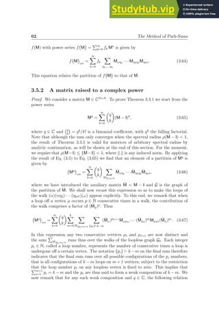
![3.5.2 A matrix raised to a complex power 63
holds:
q
k
=
X
km
km
X
km−1=0
· · ·
k2
X
k1=0
(−1)m
Qm+1
r=1 pr!
(−1)pm+1
(−q − 1) − km + pm+1
pm+1
· · ·
· · · (−1)p2
(k2 − k1 + p2)p2
(−1)p1
(k1 + p1)p1
, (3.68)
where the first sum is an indefinite sum to be evaluated at km = −q − 1. From now
on we will denote this by
P−q−1
km=0. Equation (3.68), which is independent of the value
of each individual pi, is proved by induction on m. Upon substituting this relation
into Eq. (3.65) and rearranging the order of the summations we obtain
Mq
ωα
=
∞
X
m=0
(−1)m
X
WG0;αω;m
∞
X
{pi}=0
−q−1
X
km=0
km
X
km−1=0
· · ·
k2
X
k1=0
(−M̄ω)pm+1
(−q −1)−km +pm+1
pm+1
Mωµm · · ·
· · · (−M̄µ2 )p2
(k2 − k1 + p2)p2
Mµ2α(M̄α)p1
(k1 + p1)p1
, (3.69)
where the sum
P∞
{pi}=0 =
P∞
p1=0 · · ·
P∞
pm+1=0 runs over all the loop numbers, subject
to the restriction that the loop number pi on any loopless vertex is fixed to zero. We
now evaluate the contributions from the infinite loop sums in closed form by noting
that ∞
X
pi=0
(−M̄µ)pi
(ki − ki−1 + pi)pi
pi!
= (Mµ)−(ki−ki−1)−1
, (3.70)
where we have used the fact that ρ(M̄µ) ≤ kM̄µk = kMµ − Ik ≤ kM − Ik 1.
Introducing Eq. (3.70) into Eq. (3.69) and setting k0 = 0 by definition yields the
expression
Mq
ωα
=
∞
X
m=0
(−1)m
X
WG0;αω;m
−q−1
X
km=0
km
X
km−1=0
· · ·
k2
X
k1=0
(Mω)−((−q−1)−km)−1
Mωµm · · ·
· · · (Mµ2 )−(k2−k1)−1
Mµ2α(Mα)−k1−1
. (3.71)
This expression is an m-fold nested discrete convolution. In order to convert the
discrete convolution to a product, we take the unilateral Z-transform of the above
expression with respect to n ≡ −q − 1. We obtain
Mq
ωα
= −Z−1
u
∞
X
m=0
X
WG0;αω;m
Iz−1
− Mω
−1
Mωµm · · ·
· · ·
Iz−1
− Mµ2
−1
Mµ2α
Iz−1
− Mα
−1
)
[n]
n=−q−1
, (3.72)
where z ∈ C is the Z-domain variable. Now the content of the inverse Z-transform is
a sum of walk contributions. Indeed we can see Weff
α =
Iz−1
−Mα
−1
as an effective](https://image.slidesharecdn.com/agraphtheoreticapproachtomatrixfunctionsandquantumdynamicsphdthesis-230805203656-4458b8ad/85/A-Graph-Theoretic-Approach-To-Matrix-Functions-And-Quantum-Dynamics-PhD-Thesis-73-320.jpg)
![64 The Method of Path-Sums
weight associated to vertex α. This effective weight results from the dressing of α
by all the loops off α which is performed by Eq. (3.70). Then upon remarking that
e.g. Mµ2α = wµ2α is the weight associated to edge (αµ2) from α to µ2, Eq. (3.72) is
Mq
ωα
= −Z−1
u
n X
WG0;αω
Weff
ω wωµm · · · Weff
µ2
wµ2α Weff
α
o
[n]
n=−q−1
. (3.73)
This is now in a form suitable to the use of Theorem 2.3.4. We obtain
(Mq
)ωα = −Z−1
u
X
ΠG0;αω
FG{α,...,νℓ}[ω] Mωνℓ
· · · FG{α}[ν2] Mν2α FG[α]
[n]
n=−q−1
, (3.74)
where G is the graph of {(M − I)µν}, ℓ is the length of the simple path, and
FG[α] =
h
I −
X
ΓG;α
Mαµm FG{α,...,µm−1}[µm] · · · FG{α}[µ2]Mµ2α
i−1
, (3.75)
with m the length of the simple cycle. The quantity FG[α] can itself be seen as an
effective weight associated to vertex α resulting from the dressing of α by all the
closed walks off α in G. Since a loop is a simple cycle, the dressing of the vertices
by their loops is included in FG[α] as well. This is obvious if one considers a graph
G that is reduced to a unique vertex α presenting a loop. In that case Eq. (3.75)
yields Fα[α] = [Iz−1
−Mα]−1
≡ Weff
α . For convenience we can make the loop dressing
completely explicit in Eq. (3.75) by separating the loops from the other simple cycles
FG[α] =
h
Iz−1
− Mα −
X
ΓG0;α
Mαµm FG{α,...,µm−1}[µm] · · · FG{α}[µ2]Mµ2α
i−1
, (3.76)
and note that now the sum runs over the simple cycles of the loopless graph G0.
Together with Eq. (3.74) the above Eq. (3.76) constitute the expressions presented
in Theorem 3.3.1.
Now we prove that Eqs. (3.74, 3.76) yield Mq
for any matrix by analytic continu-
ation. First, for any finite-size matrix Eqs. (3.74, 3.76) present only a finite number
of terms and must therefore converge, regardless of ρ(M − I). Second, Eqs. (3.74,
3.76) agree with the power-series Eq. (3.65) when it exists, i.e. when ρ(M − I) 1.
Third, the function Mq
and the expressions Eqs. (3.74, 3.76) are analytic. It follows
that Eqs. (3.74, 3.76) constitute the unique analytic continuation of the power-series
of Mq
. This proves Theorem 3.3.1.
3.5.3 The matrix inverse
Proof. We consider an invertible matrix M ∈ CD×D
. To prove Theorem 3.3.2 we
write the matrix inverse as M−1
=
P∞
n=0 (I − M)n
. Note that the sum only converges](https://image.slidesharecdn.com/agraphtheoreticapproachtomatrixfunctionsandquantumdynamicsphdthesis-230805203656-4458b8ad/85/A-Graph-Theoretic-Approach-To-Matrix-Functions-And-Quantum-Dynamics-PhD-Thesis-74-320.jpg)
![3.5.4 The matrix exponential 65
when the spectral radius ρ(M − I) 1; nevertheless, the result of Theorem 3.3.2 is
valid for matrices of arbitrary spectral radius by analytic continuation, see §3.5.2
above, we omit the details. Introducing an auxiliary matrix M̄ ≡ I − M, we apply
the result of Eq. (3.5) to the power series to obtain
M−1
ωα
=
∞
X
n=0
X
WG;αω;n
M̄ωηn · · · M̄η3η2 M̄η2α. (3.77)
where G is the graph of the partition of M̄. We follow the same procedure as in
§3.5.2 above and we omit the details; the result is
M−1
ωα
=
∞
X
n=0
X
WG0;αω;n
I − M̄ω
−1
M̄ωνn · · ·
I − M̄ν2
−1
M̄ν2α
I − M̄α
−1
, (3.78a)
=
∞
X
n=0
X
WG0;αω;n
(−1)n
M−1
ω Mωνn · · · M−1
ν2
Mν2α M−1
α , (3.78b)
where we have used M̄µ = I − Mµ and M̄µν = −Mµν. Eq. (3.78b) is a sum of
walk contributions with effective vertex weights Weff
µ = M−1
µ resulting from the loop
dressing of µ which occurs when Mµ 6= 0. We now use Theorem 2.3.4 and obtain
M−1
ωα
=
X
ΠG0;αω
(−1)ℓ
FG{α,...,νℓ}[ω]Mωνℓ
· · · FG{α}[ν2] Mν2α FG[α], (3.79a)
where G is the graph of {(M − I)µν}, ℓ is the length of the simple path, and
FG[α] =
h
Mα −
X
ΓG0;α
(−1)m
Mαµm FG{α,...,µm−1}[µm] · · · FG{α}[µ2]Mµ2α
i−1
, (3.79b)
with m the length of the simple cycle. Similarly to §3.5.2, we have separated the
contribution of the loops from that of the other simple cycles. This proves Theorem
3.3.2.
3.5.4 The matrix exponential
Proof. We consider a matrix M ∈ CD×D
. To prove Theorem 3.3.3 and Lemma 3.3.1,
we start from the power series expression exp(t M) =
P∞
n=0 tn
Mn
/n!. By applying
the result of Eq. (3.5) to this series we find that the partition of exp(t M) is given
by
exp(t M)ωα =
∞
X
n=0
tn
n!
X
WG;αω;n
Mωηn · · · Mη3η2 Mη2α. (3.80)](https://image.slidesharecdn.com/agraphtheoreticapproachtomatrixfunctionsandquantumdynamicsphdthesis-230805203656-4458b8ad/85/A-Graph-Theoretic-Approach-To-Matrix-Functions-And-Quantum-Dynamics-PhD-Thesis-75-320.jpg)
![66 The Method of Path-Sums
with G the graph of the partition of M. Following the same procedure as in §3.5.2,
we make the loop of the walks appear explicitly
exp(t M)ωα =
∞
X
n=0
tn
n!
n
X
m=0
X
WG0;αω;m
X
{pi}⊢n−m
(Mω)pm+1
Mωµm· · · (Mµ2 )p2
Mµ2α(Mα)p1
, (3.81)
where the again loop numbers satisfy
Pm+1
i=1 pi = n − m, with the restriction that
the loop numbers on any loopless vertices are fixed to zero. Such a sequence is said
to form a weak composition of n − m. We now note that for any weak composition
of n − m, the following identity holds:
1
p1! p2! · · · pm+1!
Z t
0
dtm · · ·
Z t2
0
dt1 (t − tm)pm+1
· · · (t2 − t1)p2
tp1
1 =
tn
n!
. (3.82)
This result – which does not depend on the value of each individual pi – is straight-
forwardly proved by induction on m. By substituting this identity into Eq. (3.81)
and rearranging the order of summations we obtain
exp t M
ωα
= (3.83a)
∞
X
m=0
X
WG0;αω;m
∞
X
{pi}=0
Z t
0
dtm · · ·
Z t2
0
dt1
(t − tm)Mω
pm+1!
pm+1
Mωµm· · ·
(t2 − t1)Mµ2
p2!
p2
Mµ2α
t1Mα
p1!
p1
,
=
∞
X
m=0
X
WG0;αω;m
Z t
0
dtm · · ·
Z t2
0
dt1 e(t−tm)Mω
Mωµm · · · e(t2−t1)Mµ2 Mµ2α et1Mα
. (3.83b)
This intermediate result proves Lemma 3.3.1. In order to continue, we note that
this expression is an m-fold nested convolution. To convert the convolution to a
product we take the Laplace transform of both sides:
L
exp(t M)ωα
=
∞
X
m=0
X
WG0;αω;m
L
fω(t)
Mωµm · · · L
fµ2 (t)
Mµ2α L
fα(t)
, (3.84)
=
∞
X
m=0
X
WG0;αω;m
[sI − Mω]−1
Mωµm · · · [sI − Mµ2 ]−1
Mµ2α [sI − Mα]−1
, (3.85)
where the second line follows on noting the result L
exp(tMµ)
=
sI − Mµ
−1
. As
in the previous sections, we remark that Eq. (3.85) is a sum of walk contributions
with an effective vertex weight of Weff
µ = [sI − Mµ]−1
. On using Theorem 2.3.4 to](https://image.slidesharecdn.com/agraphtheoreticapproachtomatrixfunctionsandquantumdynamicsphdthesis-230805203656-4458b8ad/85/A-Graph-Theoretic-Approach-To-Matrix-Functions-And-Quantum-Dynamics-PhD-Thesis-76-320.jpg)
![3.5.5 The matrix logarithm 67
turn Eq. (3.85) into a path-sum, we obtain
L
exp t M
ωα
=
ℓmax
X
ℓ=0
X
ΠG0;αω;ℓ
FG{α,...,νℓ}[ω] Mωνℓ
· · · FG{α}[ν2] Mν2α FG[α] , (3.86a)
FG[α] =
h
sI − Mα −
X
ΓG0;α
Mαµm FG{α,...,µm−1}[µm] · · · FG{α}[µ2]Mµ2α
i−1
, (3.86b)
where ℓ and m are the length of the simple path and of the simple cycle, respectively.
In this expression, the contribution from the loops is explicitly separated from that
of the other simple cycles.
3.5.5 The matrix logarithm
Proof. In this section, we consider a matrix M ∈ CD×D
with no eigenvalue on
the negative real axis. To prove Theorem 3.3.4 we write the matrix logarithm as
log M = −
P∞
n=1(I − M)n
/n. This series only converges when the spectral radius
ρ(M − I) 1; nevertheless, the result of Theorem 3.3.4 is valid for matrices of
arbitrary spectral radius by analytic continuation. We introduce the auxiliary matrix
M̄ ≡ I − M and rewrite the power series as
log M
ωα
= −
∞
X
n=1
1
n
X
WG0;αω;n
M̄ωνn · · · M̄ν3ν2 M̄ν2α, (3.87a)
= −
∞
X
n=1
1
n
n
X
m=0
X
WG0;αω;m
X
{pi}⊢n−m
M̄ω
pm+1
M̄ωµm
· · · M̄µ2
p2
M̄µ2α M̄α
p1
, (3.87b)
with G the graph of the partition of M̄. The second equality is obtained by making
the loops explicit through the same procedure as in §3.5.2. Just as in the previ-
ous sections, the loop numbers form a weak composition of n − m. For any such
composition, the following identity holds:
1
n
=
Z 1
0
xm−1
xp1
xp2
· · · xpm+1
dx. (3.88)
This identity allows the contributions from the infinite loop sums in Eq. (3.87b) to
be evaluated in closed form. By restructuring the double summation we obtain
log M
ωα
= −δωα
Z 1
0
M̄α
I − xM̄α
−1
dx (3.89)
−
∞
X
m=1
X
WG0;αω;m
Z 1
0
xm−1
I − xM̄ω
−1
M̄ωµm · · ·
I − xM̄µ2
−1
M̄µ2α
I − xM̄α
−1
dx,](https://image.slidesharecdn.com/agraphtheoreticapproachtomatrixfunctionsandquantumdynamicsphdthesis-230805203656-4458b8ad/85/A-Graph-Theoretic-Approach-To-Matrix-Functions-And-Quantum-Dynamics-PhD-Thesis-77-320.jpg)
![68 The Method of Path-Sums
where we have written
I − xM̄µ
−1
for
P∞
p=0(xM̄µ)p
and δωα is a Kronecker delta.
Note that the first part of this expression – which represents contributions from
walks consisting entirely of loops – has a slightly different structure than the second
part, owing to the absence of the term with zero loops when ω = α. Just as for
the previously obtained matrix functions, the integrand of Eq. (3.89) is a sum of
walk contributions with effective vertex weights Weff
µ =
I − xM̄µ
−1
. On using the
path-sum formula, Theorem 2.3.4, Eq. (3.89) transforms to
log M
ωα
= (3.90a)
Z 1
0
dx x−1
(I − FG[α]) , ω = α,
−
X
ΠG0;αω
Z 1
0
dx xℓ−1
FG{α,...,νℓ}[ω]M̄ωνℓ
· · · FG{α}[ν2] M̄ν2α FG[α], ω 6= α,
where ℓ the length of the simple path and
FG[α] =
h
I − xM̄α −
X
ΓG0;α
xm
M̄αµm FG{α,...,µm−1}[µm] · · · M̄µ3µ2 FG{α}[µ2]M̄µ2α
i−1
,
(3.90b)
with m the length of the simple cycle. Note that we have again explicitly separated
the contribution of the loops from that of the other simple cycles. Theorem 3.3.4 is
now directly obtained upon replacing M̄ by I − M.
3.6 Summary and Outlook
The method of path-sums is based on three main concepts: firstly, the partitioning
of a discrete matrix M into an ensemble of submatrices whose dimensionalities can
be freely chosen; secondly, the mapping between multiplication of M and walks on
a graph G whose edge pattern encodes the structure of M; and thirdly, the exact
closed-form resummation of certain classes of walks on G through the dressing of
vertices by cycles. By combining these concepts, any partition of a function of a
finite matrix f M
– whose entries do not necessarily have to commute with one
another – can be exactly evaluated in a finite number of steps, provided the required
inverse transforms are analytically available.
Using a directed graph to encode the structure of a matrix allows any structure
and symmetries that the matrix possesses to be easily recognized and exploited.
We thus expect the method of path-sums to have widespread applications in, for
example, the study of Markov chains and quantum many-body physics, where the
relevant matrix – the many-body Hamiltonian – is both sparse and highly structured.
In Chapters 4 and 5 we present applications of the method to the study of quantum
dynamics.
A major issue which we have not addressed so far is that of the truncation of
a path-sum. On highly connected graphs the number of simple paths and simple](https://image.slidesharecdn.com/agraphtheoreticapproachtomatrixfunctionsandquantumdynamicsphdthesis-230805203656-4458b8ad/85/A-Graph-Theoretic-Approach-To-Matrix-Functions-And-Quantum-Dynamics-PhD-Thesis-78-320.jpg)
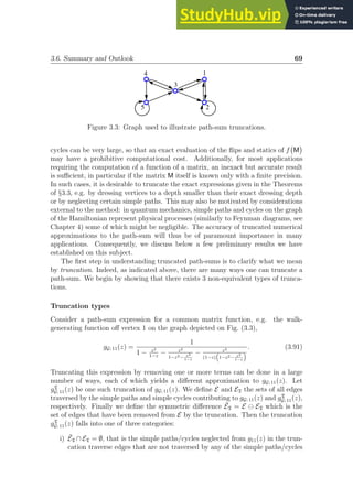
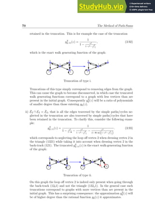
![3.6. Summary and Outlook 71
iii) ĒT ∩ ET 6= ∅ and ĒT ∩ ET 6= ĒT, i.e. the truncation is a mixture of the above
two types of truncations. The degree gT
G (z) can be higher or lower than that
of gG(z).
This brief analysis applies generally to any truncation of a path-sum and thus shows
that truncating path-sums is not simple: in particular it does not necessarily cor-
responds to zeroing out elements of the matrix M whose function f(M) is being
calculated.
Remark 3.6.1 (Simulating non-Markovian dynamics). Truncations of type ii) could
perhaps be used to simulate non-Markovian behaviors in physical systems. Indeed,
such truncations correspond to neglecting edges depending on their context (i.e.
inside of which simple path/cycle is a vertex being dressed). In Chapter 4 we
show that in the context of quantum dynamics, each edge of the graph representing
the configurations available to a physical system correspond to a physical process
provoking a change in the state of the system. Then walks, simple paths and simple
cycles represent succession of physical processes occurring in the system, i.e. its
histories. In this picture, truncations of type ii) are equivalent to certain physical
processes taking place or not depending on the previous history of the system,
something characteristically non-Markovian.
Behavior of truncated path-sums
The question of the quality of the approximation obtained by truncating a path-sum
remains largely open. A naive approach to this question based on evaluating the
number of walks taken into account in a truncated path-sum encounters a variety
of problems: i) the number of walks taken into account and neglected are both
typically infinite; and ii) the weights of the walks might play a dominant role.
A more promising alternative consists of constraining the weight of fully dressed
simple paths and simple cycles based on their length. In the region of convergence of
the power-series representation of f(M) this is straightforward. To see this, consider
the power-series expansion f(z) =
P
n fnzn
with convergence radius ρf . Let M ∈
CD×D
, {Mαω} a partition of M with graph G and define m = maxα,ω kMαωk. Clearly
the weight W[p] of a fully dressed prime p ∈ ΠG ∪ ΓG of length ℓ(p) and with end
points µ, ν in the path-sum expression of f(M) is upper bounded by the total weight
carried by all the walks with end points µ, ν and of length greater than or equal to
ℓ(p), i.e.
W[p] ≤
X
n≥ℓ(p)
|WG; µν|(n)fnmn
, (3.94)
where we assumed existence of the power-series. This holds as long as m × b ρf
with b the maximum eigenvalue of the largest connected component of G containing
vertices µ and ν.
The result of Eq. (3.94) works well for entire functions, predicting for example a
super exponential decay of W[p] as a function of ℓ(p) for f(z) = ez
on path-graphs](https://image.slidesharecdn.com/agraphtheoreticapproachtomatrixfunctionsandquantumdynamicsphdthesis-230805203656-4458b8ad/85/A-Graph-Theoretic-Approach-To-Matrix-Functions-And-Quantum-Dynamics-PhD-Thesis-81-320.jpg)
![72 The Method of Path-Sums
6
. This approach fails however for many functions of interest, e.g. log(z), zq
etc.,
for which the region of convergence of the power-series representation of f(M) is
finite. In such situations it may be possible to establish the decay of fully dressed
primes from more general arguments. Recent research [80, 81, 82, 83] showed that
the entries f M
ij
of certain matrix functions decay exponentially with the length of
the shortest simple path between the vertices that correspond to entries Mii and Mjj.
Furthermore, Prof. Benzi and coworkers have recently extended these results to the
norm of the statics and flips of any tensor-partition of f M
[84]. We are convinced
that these results are related with the weight of individual prime walks, such as is
the case for entire functions. For matrices which are deterministically known, the
demonstration of such a link has resisted our attempts so far. For random matrices
however, the results of Chapter 5 establish that on average the weight of a fully
dressed simple path decays exponentially with its length. In turn this implies that
on average, matrix functions are exponentially localised.
6
This result is closely related to the decay away from the diagonal of exp(M) with M tridiagonal,
established by [79].](https://image.slidesharecdn.com/agraphtheoreticapproachtomatrixfunctionsandquantumdynamicsphdthesis-230805203656-4458b8ad/85/A-Graph-Theoretic-Approach-To-Matrix-Functions-And-Quantum-Dynamics-PhD-Thesis-82-320.jpg)

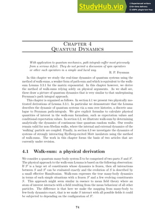
![4.1.1 Model system and general approach 75
In practice, the walk-sum method divides the matrix representing the time evolu-
tion operator of a finite-dimensional quantum system into small pieces. These pieces
are called conditional evolution operators and are introduced in section 4.1.1, where
we describe the general approach of the method. In section 4.1.2 we derive an equa-
tion that allows one to calculate any conditional evolution operator and therefore
any desired piece of the full evolution operator. We then show in section 4.1.3 that
the generation of conditional evolution operators can be represented by walks on a
graph. This facilitates the evaluation of the walk-sum expression. In section 4.1.4
we give the expression of the conditional evolution operators in the Laplace domain.
Finally, we demonstrate how the method allows one to evaluate expectation values
and conditional expectation values in §4.1.5.
4.1.1 Model system and general approach
We consider a quantum many-body system S that is described by a time-independent
Hamiltonian H and comprised of N physical constituents. The state space of the
kth constituent is spanned by dk internal levels, where dk can be different for every
k. Let {|iki} be an orthonormal basis of length dk associated with constituent k,
and Pk,i = |ikihik| be the projector onto state |iki. Next we split the system S
into two parts S and S′
. Here constituent s is taken to be S, and all remaining
constituents are grouped in S′
. Note that constituent s can be comprised of one or
several physical particles. We define so-called projector-lattices
εµ = ⊗k∈S′ Pk,ik
⊗ Is =
Acts on S′
z }| {
|µihµ| ⊗
Acts on S
z}|{
Is (4.1)
that are projection operators in the state space of the full system S. The index µ
is a short-hand notation for the configuration onto which S′
is projected and Is is
the identity operator on S. There is a total of
QN
k6=s dk different projector-lattices
corresponding to all possible combinations of projectors Pk,ik
. Projector-lattices are
themselves orthogonal projectors and the ensemble of all possible projector-lattices
is closed,
ενεµ = δν,µ εν,
X
ν
εν = I, (4.2)
where I is the identity operator on the state-space of the whole many-body system
S. Next we partition the time evolution operator U = exp[−iHt] (from now on we
set ~ = 1) into submatrices with projector lattices,
ενU(t)εµ = ⊗k∈S′ Tk,ik←jk
⊗ Uν←µ(t) = |νihµ|
| {z }
Acts on S′
⊗ Uν←µ(t)
| {z }
Acts on S
. (4.3)
Here Tk,i←j = |ikihjk| denotes a transition operator in subsystem k, and Uν←µ(t) is
a so-called conditional evolution operator that is represented by a (small) ds × ds](https://image.slidesharecdn.com/agraphtheoreticapproachtomatrixfunctionsandquantumdynamicsphdthesis-230805203656-4458b8ad/85/A-Graph-Theoretic-Approach-To-Matrix-Functions-And-Quantum-Dynamics-PhD-Thesis-85-320.jpg)
![76 Quantum Dynamics
matrix. Uν←µ(t) generates the time evolution of subsystem S provided that (i) the
remaining many-body system S′
was initially in configuration |µi, and (ii) the state
of S′
at time t is given by |νi. The closure relation in Eq. (4.2) implies that the full
time evolution operator U(t) can be represented in terms of conditional evolution
operators,
U(t) =
X
ν, µ
n
|νihµ|
| {z }
Acts on S′
⊗ Uν←µ(t)
| {z }
Acts on S
o
. (4.4)
In the language of Chapter 3, the ensemble {Uν←µ(t)} forms a tensor product parti-
tion of U(t). The method of walk-sums allows one to compute conditional evolution
operators efficiently, i.e. in a number of operations scaling polynomially in the
number of involved particles, and independently of one another. If in a particular
physical problem only a small subset of all possible configurations of S′
is relevant,
then our approach allows one to approximate the full time evolution with a moderate
computational effort.
4.1.2 Derivation of the conditional evolution operators
In this section we derive an explicit expression for conditional evolution operators
using two different approaches: the first emphasises their interpretations in terms
of histories of the system and the second, simpler, relies on existing results from
perturbation theory.
Conditional evolution operators as superpositions of histories
We begin with writing the time evolution operator U(t) of the complete system S
as a succession of infinitesimal time evolutions
U(t) = exp[−iHt] = lim
δt→0
M
Y
n=1
δU = lim
δt→0
M
Y
n=1
X
α
εα δU , (4.5)
where δU = I − iHδt is the infinitesimal evolution operator from (n − 1)δt to nδt
and M = t/δt. In the last step in Eq. (4.5) we inserted the closure relation for
projector lattices [see Eq. (4.2)]. In the following, we derive explicit expressions
for the conditional time evolution operators Uν←µ(t) by a re-summation of terms
arising in ενU(t)εµ. Let us first focus on ενU(t)εν, and in particular the term where
all intermediate projector lattices εα in Eq. (4.5) are all equal to εν,
U(0)
ν = εν
M
Y
n=1
{εν δU εν = εν δU εν δU . . . εν δUεν. (4.6)
The physical meaning of this term is the following. First S′
is projected into config-
uration ν, then δU evolves the full system S from 0 to δt. Then εν projects S′
onto
configuration ν, followed by a time evolution of S for δt, and so on. In the limit](https://image.slidesharecdn.com/agraphtheoreticapproachtomatrixfunctionsandquantumdynamicsphdthesis-230805203656-4458b8ad/85/A-Graph-Theoretic-Approach-To-Matrix-Functions-And-Quantum-Dynamics-PhD-Thesis-86-320.jpg)
![4.1.2 Derivation of the conditional evolution operators 77
δt → 0, S′
is frozen by continuous (Zeno) measurements of |νihν| and S evolves
freely under the influence of S′
in configuration ν. We find
lim
δt→0
U(0)
ν = lim
δt→0
M
Y
n=1
(εν − i ενHενδt) = uν(t, 0), (4.7)
where
uν(t, t′
) = εν e−i εν Hεν (t−t′)
(4.8)
is a so-called Zeno evolution operator that evolves S between times t and t′
while S′
is frozen in configuration |νi. Zeno-evolution operators obey the following relations
uνuµ = 0 if ν 6= µ, ενuν = uνεν = uν, and u†
νuν = uνu†
ν = εν. (4.9)
Next we discuss the projection ενU(t)εµ for µ 6= ν and focus on those terms that are
of the form
U(1)
νµ = εν δU εν δU . . . εν δU εν δU εµ δU εµ δU . . . εµ δU εµ (4.10a)
= −iδt εν δU εν δU . . . εν δU εν
| {z }
= X (M−M′ times δU)
ενHεµ εµ δU εµ δU . . . εµ δU εµ
| {z }
= Y (M′−1 times δU)
, (4.10b)
where we employed εν δU εµ = −iδt ενHεµ. Now let t = Mδt and t′
= M′
δt. The
term U
(1)
νµ can be interpreted as follows. Initially S′
is projected into state |µi and
we observe that limδt→0 Y = uµ(t′
, 0). This is the Zeno evolution operator for S
that keeps S′
static in state |µi between 0 and t′
. Then the subsystem S′
makes
a jump from configuration |µi to configuration |νi [term ενHεµ], followed by the
evolution of S between t′
and t with S′
frozen in state |νi [term X in Eq. (4.10a)
fulfils limδt→0 X = uµ(t, t′
)]. Note that the limit t → 0 cannot be taken directly in
U
(1)
νµ , since there are M → ∞ (δt → 0) similar terms appearing in ενU(t)εµ that
differ from U
(1)
νµ only in the position of the jump operator ενHεµ, i.e. the time t′
at
which S′
makes the transition µ → ν. Summing over all these terms and taking the
limit t → 0 yields
lim
δt→0
M
X
q=1
−iδt X(t, qδt) H Y(qδt − δt, 0) = −i
Z t
0
uν(t, t′
) H uµ(t′
, 0)dt′
, (4.11)
and the integral is thus a continuous sum over the time for the jump µ → ν to
occur. The full expansion of ενU(t)εµ also contains terms with an arbitrary number
of intermediary configurations ηq between the initial and final configurations µ and
ν, respectively. For each of these configurations, the jump ηq → ηq+1 can occur at](https://image.slidesharecdn.com/agraphtheoreticapproachtomatrixfunctionsandquantumdynamicsphdthesis-230805203656-4458b8ad/85/A-Graph-Theoretic-Approach-To-Matrix-Functions-And-Quantum-Dynamics-PhD-Thesis-87-320.jpg)
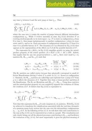
![4.1.3 Representing the time evolution on a graph 79
walks, simple paths and simple cycles as system histories.
Perturbation theory
We now provide a simpler and shorter alternative derivation of the conditional evo-
lution operators from a perturbative expansion of the time evolution operator in
the transitions undergone by S′
. We start with the well-known expression (see, e.g.,
Complement AI.2 in [85]), called Dyson series for the evolution operator. In time-
dependent perturbation theory, it is used to describe the dynamics of a system with
Hamiltonian H0 in the presence of a perturbation V
U(t, 0) = exp[−i(H0 + V)t] = exp[−iH0t]+ (4.15)
∞
X
n=1
i−n
Z t
0
Z tn
0
. . .
Z t2
0
e−iH0(t−tn)
V e−iH0(tn−tn−1)
V . . . e−iH0t1
dt1 . . . dtn.
In order to establish Eq. (4.12) via Eq. (4.15), we expand the Hamiltonian H in terms
of the complete set of projector-lattices in Eq. (4.2) and obtain H = H0 + V, where
H0 =
X
ν
ενHεν, V =
X
ν6=µ
ενHεµ. (4.16)
If these expressions are introduced in Eq. (4.15), the orthogonality of the projector
lattices directly yields the result in Eq. (4.12). From this, the mixed product prop-
erty of the tensor-product gives Eq. (4.14). This indicates another interpretation for
the result of Eq. (4.14): the transitions undergone by S′
can be seen as perturbations
affecting the evolution of S.
4.1.3 Representing the time evolution on a graph
The sum over the intermediary configurations ηq in Eq. (4.14) can be interpreted as
a sum over the histories of S′
, a history being a succession of configurations adopted
by S′
from 0 to time t. To visualise the histories, we construct a graph G as follows:
i) For each configuration ν available to S′
, draw a vertex vν.
ii) For each non-zero flip, i.e. when S′
is allowed to make a transition between two
specific configurations µ and ν, draw an edge between vµ and vν.
Because of i), we call G the configuration graph of the system. Now we can see
that a multiplication by e−iHν τ
in Eq. (4.14) represents the evolution of S while S′
is stationary at vertex vν during time τ. A multiplication by Hν←µ in Eq. (4.14)
corresponds to an instantaneous move of S′
along the edge vµ → vν. Consequently,
the histories of S′
appear as walks on G and their superposition is obtained as the
sum over all the walks, in complete analogy with the Feynman path-integrals. If
the system had continuous degrees of freedom, the sum over histories, that is the
sum over the walks, would become an integral over histories which corresponds to
an integral over the walks, i.e. a Feynman path-integral. An equivalent to the](https://image.slidesharecdn.com/agraphtheoreticapproachtomatrixfunctionsandquantumdynamicsphdthesis-230805203656-4458b8ad/85/A-Graph-Theoretic-Approach-To-Matrix-Functions-And-Quantum-Dynamics-PhD-Thesis-89-320.jpg)
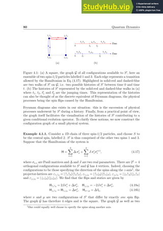
![4.1.4 Evaluation of conditional evolution operators 81
examples for histories of S′
, two walks and the equivalents of Feynman diagrams are
all represented in Fig. 4.1.
In order to make the superposition of histories manifest in the expression for
Uν←µ(t), we relabel the sum over intermediary configurations into a sum over all the
walks on G. If the initial and final configurations of S′
appearing in Eq. (4.14) are
respectively µ and ν, then the relevant walks all start on vertex vµ and terminate
on the vertex vν. The conditional evolution operator Uν←µ is therefore
Uν←µ(t) = e−iHν t
δµ,ν +
∞
X
n=1
i−n
X
WG;νµ;n
(4.19)
×
Z t
0
Z tn
0
. . .
Z t2
0
e−iHν (t−tn)
Hν←ηn e−iHηn (tn−tn−1)
Hηn←ηn−1 . . . e−iHµt1
dt1 . . . dtn,
where WG;νµ;n is the ensemble of walks of length n on G from vµ to vν. Eq. (4.19) is
the walk-sum Lemma 3.3.1 applied to the matrix exponential exp[−iHt].
4.1.4 Evaluation of conditional evolution operators
Conditional evolution operators are most conveniently evaluated in the Laplace do-
main, because this transformation turns the nested convolutions in Eq. (4.19) into
a product of matrices. Let M̃µ(s) = L exp[−iHµt]
= (sIs + iHµ)−1
be the element-
wise Laplace transform of exp[−iHµt] with s the Laplace domain variable. It follows
that the Laplace transform of a conditional evolution operator is given by
Ũν←µ(s) = M̃ν(s)δµ,ν +
∞
X
n=1
X
WG;νµ;n
i−n
M̃ν(s) Hν←ηn . . . Hη1←µ M̃µ(s). (4.20)
This is the expression we use in computations. It only involves multiplications and
additions of ds × ds matrices. Considering the case where all the M̃µ(s) can be
obtained analytically, we remark that the matrix elements of the M̃µ(s) are ratios
of polynomials in s. The roots of the denominator polynomial are −iλµ with λµ an
eigenvalue of Hµ. This is therefore also true for any element of the sum in Eq. (4.20)
and performing the inverse transform into the time-domain can be done according
to the formula
Uν←µ(t) =
X
µ
Res[est
Ũν←µ(s), −iλµ], (4.21)
where Res[f(s), λ] denotes the residue of f(s) at λ. In all practical situations the
infinite sum in Eq. (4.19) is truncated at some order K. With this approximation
only walks of length n ≤ K are taken into account. It is important to establish the
convergence properties of such truncated walk-sums.](https://image.slidesharecdn.com/agraphtheoreticapproachtomatrixfunctionsandquantumdynamicsphdthesis-230805203656-4458b8ad/85/A-Graph-Theoretic-Approach-To-Matrix-Functions-And-Quantum-Dynamics-PhD-Thesis-91-320.jpg)
![82 Quantum Dynamics
Convergence
Consider the contribution to Uν←µ(t) of the walks of length exactly K, denoted
U
[K]
ν←µ(t). A naive bound for the norm of this quantity is
U[K]
ν←µ(t) ≤ |WG;νµ;K|
(Ω t)K
K!
, (4.22)
with Ω = maxn{Hηn+1←ηn } and |WG;νµ;K| is the number of walks of length K on
G between vertices vν and vµ. It is noteworthy that |WG;νµ;K| is bounded by a
polynomial in the number N of particles of the system, see below. The bound
demonstrates that provided S comprises a finite number of particles, the series of
Eq. (4.19) is absolutely and uniformly convergent for any finite time.
Computational cost: polynomial scaling in N
In this section we show that the number of floating point operations required to
approximate a conditional evolution operator to order K scales polynomially in the
number of particles N of the system. For simplicity and without loss of generality,
we assume that all particles have d internal levels and that S contains p particles,
and thus ds = dp
. The evaluation of a single walk of length K to a conditional
evolution operator requires 2K +1 multiplications of ds ×ds matrices (K statics and
K +1 flips), i.e. ∼ 2Kd3
s operations. Then all the walk contributions must be added
together. This represents an additional |WG;νµ;K|d2
s operations. The total number
NK of operations required to obtain Uµ←ν at order K is therefore
NK = (2Kd3
s + d2
s)|WG;νµ;K|. (4.23)
The remaining task is to derive an upper bound for |WG;νµ;K|.
Suppose that the flips of the Hamiltonian H of S [see Eq. (4.13)] are only non-zero
for those configurations µ and ν of S′
where at most q particles change their state
in a transition from µ to ν. For example, the expressions for the flips in Eqs. (4.18)
and (4.78) demonstrate that the Hamiltonians in Eqs. (4.17) and (4.75) have q = 1.
In fact, most of the common Hamiltonians have q = 1, 2. With p particles in S there
are N − p particles in S′
, and thus there are N−p
q
ways to choose which q particles
among N − p undergo a transition. Furthermore, for each particle that changes a
state there are at most d − 1 possible basis states available for the transition. In
total, there are thus at most V N−p
q
(d − 1)q
configurations directly accessible
to S′
from any given one. By construction of G, this is also an upper-bound on the
number of vertices that share an edge with any given vertex on G. It follows that
there are at most V K
walks of length K attached to any vertex of G, and thus we
find
|WG;νµ;K| N−p
q
K
(d − 1)qK
, (4.24)
which scales polynomially in N − p for small q.
Remark 4.1.1 (Spin-1/2 systems). The upper-bound Eq. (4.24) is very loose and](https://image.slidesharecdn.com/agraphtheoreticapproachtomatrixfunctionsandquantumdynamicsphdthesis-230805203656-4458b8ad/85/A-Graph-Theoretic-Approach-To-Matrix-Functions-And-Quantum-Dynamics-PhD-Thesis-92-320.jpg)
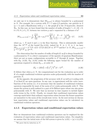
![84 Quantum Dynamics
where |ψs(0)i is the initial state of S. Note, all the relations of this sections are easily
extended to more general initial pure states
P
µ cµ|µi ⊗ |ψs(0)i upon introducing a
sum over µ as appropriate. The state vector of the full system can then be obtained
via Eq. (4.4) and is given by
|ψ(t)i = U(t)|ψ(0)i =
X
ν
n
|νi ⊗ |ψs(t)iν←µ
o
, (4.27)
where |ψs(t)iν←µ = Uν←µ(t)|ψs(0)i is a piece of the wavefunction of the full system.
Any mean value of an observable O can be calculated via Eq. (4.27). With the
definition εν′ Oεν = |ν′
ihν| ⊗ Oν′ν, we find
hOi = hψs(0)|
X
ν′
,ν
U†
µ→ν′ Oν′ν Uν←µ |ψs(0)i. (4.28)
In this expression U†
µ→ν′ = Uν′←µ
†
. It follows that any expectation value of an
observable O can be computed directly from conditional evolution operators if O is
expanded in the projector lattice basis εν.
Next we investigate in more detail the meaning of the piece |ψs(t)iν←µ = Uν←µ(t)|ψs(0)i
of the full state vector. To this end, we write the projection of |ψ(t)i onto the range
of εν as
εν |ψ(t)i = |νi ⊗ |ψs(t)iν←µ =
ds
X
ℓ=1
αℓ |νℓsi, (4.29)
where the probability amplitudes αℓ of state |νℓsi (S′
in configuration ν, S in state
|ℓsi) are determined by Uν←µ(t). This shows that Uν←µ(t) directly evolves the pro-
jection of the full state vector |ψ(t)i onto a ds-dimensional subspace corresponding
to S′
in configuration ν, as shown in Fig. 4.2. We emphasise that conditional evo-
lution operators are submatrices of U [see Eq. (4.4)] and therefore not necessarily
unitary. It follows that Uν←µ(t) does not generally conserve the norm of |ψs(0)i.
Indeed, Eq. (4.29) implies that the norm of |ψs(t)iν←µ is given by the probability of
finding S′
in configuration ν at time t, knowing that it was initially in configuration
µ,
hψs(0)| U†
µ→ν(t) Uν←µ(t) |ψs(0)i = hενit. (4.30)
We now turn to conditional expectation values and show that some of them can
be computed directly via a single conditional evolution operator. To this end, we
note that the expectation value of an arbitrary operator Os acting on S with respect
to |ψs(t)iν←µ is given by
hψs(0)| U†
µ→ν(t) Os Uν←µ(t) |ψs(0)i = hOsενit, (4.31)
where hOsενit is the expectation value of Osεν at time t. Eqs. (4.30, 4.31) directly
yield the conditional expectation value hOs/νi of Os, knowing that S′
, initially in](https://image.slidesharecdn.com/agraphtheoreticapproachtomatrixfunctionsandquantumdynamicsphdthesis-230805203656-4458b8ad/85/A-Graph-Theoretic-Approach-To-Matrix-Functions-And-Quantum-Dynamics-PhD-Thesis-94-320.jpg)
![4.1.5 Expectation values and conditional expectation values 85
ÈΨH0L
UHtLÈΨH0L
¶
`
Ν
¶
`
Μ
UΜ¬ΜHtLÈΨsH0L
UΝ¬ΜHtLÈΨsH0L
Figure 4.2: The conditional evolution operator Uν←µ(t) evolves only the projection
of the full evolution U(t)|ψ(0)i onto the subspace of the full state-space that cor-
responds to S′
being in configuration ν. Note that in this picture, S′
is initially in
configuration µ.
configuration µ, is in configuration ν at time t, 3
hOs/νi =
hOsενi
hενi
=
hψs(0)| U†
µ→ν(t) Os Uν←µ(t) |ψs(0)i
hψs(0)| U†
µ→ν(t) Uν←µ(t)|ψs(0)i
. (4.32)
Finally, Eqs. (4.2) and (4.32) imply that the full set of conditional probabilities allows
one to compute the mean value of an operator acting on S,
P
νhOs/νihενi = hOsi.
We use the preceding results in sections §4.2 and §4.3, where we apply the walk-sum
method to study continuous-time coined quantum random walks and the dynamics
of strongly interacting Rydberg-excited Mott insulators. But first, we give a very
simple example to illustrate the method.
Example 4.1.2 (Dynamics of 3 spins). Consider a small 1D chain with 3 spin-1/2
particles evolving according to the Hamiltonian in Eq. (4.17). Suppose that initially
all three spins are up along z, i.e. |ψ(0)i = | ↑1↑2↑3i and suppose that we are
interested in the time evolution of the conditional expectation value h↑2 / ↑1↑3i.
This is the probability for spin 2 to be up along z knowing the other 2 spins are up
along z. To implement walk-sum, we take S to be the spin 2 and S′
comprises spins
1 and 3. Similarly to the example of section 4.1.3, we choose the configurations of
S′
to specify the direction of these spins along the z-axis and obtain the flips and
statics of Eq. (4.18). The graph G is the square represented in Fig. 4.1. According
3
The fact that hOsενi/hενi is indeed the conditional expectation value follows from [Os, εν] = 0
and ε2
ν = εν [86].](https://image.slidesharecdn.com/agraphtheoreticapproachtomatrixfunctionsandquantumdynamicsphdthesis-230805203656-4458b8ad/85/A-Graph-Theoretic-Approach-To-Matrix-Functions-And-Quantum-Dynamics-PhD-Thesis-95-320.jpg)
![86 Quantum Dynamics
0 1 2 3 4 5 6 7
0.975
0.9875
1
JtΠ
X
z
2
z
1
z
3
0 1 2 3 4 5 6 7
0.975
0.9875
1
JtΠ
X
z
2
z
1
z
3
Figure 4.3: Top figure: evolution of h↑2 / ↑1↑3i evaluated by walk-sum at order 2
(solid blue line) compared to the exact solution (dashed red line). Bottom figure:
evolution of h↑2 / ↑1↑3i evaluated by walk-sum at order 4 (solid black line) compared
to the exact solution (dashed red line). Note that order 4 is the next non-zero order
after order 2. Parameters: J/∆ = 4.
to Eq. (4.32), the quantity h↑2 / ↑1↑3i is given by
h↑2 / ↑1↑3i =
hψs(0)|U†
↑1↑3→↑1↑3
P↑2 U↑1↑3←↑1↑3 |ψs(0)i
hψs(0)|U†
↑1↑3→↑1↑3
U↑1↑3←↑1↑3 |ψs(0)i
, (4.33)
where P↑2 = |↑2ih↑2 | and |ψs(0)i = |↑2i is the initial state of subsystem S. Con-
sidering the closed walks off vertex v↑1↑3 on G and keeping only walks of length 2 or
less, the conditional evolution operator in the Laplace domain Ũ↑1↑3←↑1↑3 is given by
Ũ↑1↑3←↑1↑3 (s) ≃
Walk of length 0
z }| {
M̃↑1↑3 + (−i∆)2
Two walks of length 2
z }| {
M̃↑1↑3 (M̃↓1↑3 + M̃↑1↓3 )M̃↑1↑3 , (4.34)
where the factor (−i∆)2
comes from the flips. The two walks of length two taken
into account here are those highlighted by solid-red and dashed-blue lines in Fig. 4.1.
In Fig. 4.3 we compare the walk-sum result for the time evolution of h↑2 / ↑1↑3i to
the exact result. For short times Jt . 3π, the agreement between the walk-sum
estimation of h↑2 / ↑1↑3i at order 2 and the exact result is excellent. Differences
appear for Jt 3π and grow larger with time. At order 4, which is the next non-zero
order, the difference between the walk-sum estimation and the exact result does not
exceed 5 × 10⁻³
for t up to Jt ∼ 7π, which represents a relative error of less than
0.5%. As a comparison, the method of path-sums yields Ũ↑1↑3←↑1↑3 (s) exactly as
Ũ↑1↑3←↑1↑3 (s) =
h
sI − ∆σx − 2Jσz (4.35)
− 2∆2
[sI − ∆σx − ∆2
B]−1
− 2∆4
AB[sI − ∆σx − ∆2
B]−1
i−1
,](https://image.slidesharecdn.com/agraphtheoreticapproachtomatrixfunctionsandquantumdynamicsphdthesis-230805203656-4458b8ad/85/A-Graph-Theoretic-Approach-To-Matrix-Functions-And-Quantum-Dynamics-PhD-Thesis-96-320.jpg)
![4.1.6 Two state vector formalism 87
where A = [sI − ∆σx]−1
and B = [sI − ∆σx + 2Jσz − ∆2
A]−1
.
4.1.6 Two state vector formalism
To conclude the discussion devoted to the physical interpretation of the conditional
evolution operators, we demonstrate that the Aharonov-Bergmann-Lebowitz rule of
the Two State Vector Formalism [87, 88] can be naturally expressed with conditional
evolution operators. This formalism was developed by Aharonov and coworkers to
answer the following question. A quantum system initially in state |ψ0i at t0 is
measured at a later time tf in state |ψf i. What is the probability to find this
system in state |ψqi at any time t ∈ [t0, tf ]? The conditional probability of finding
|ψqi at t knowing the system starts in |ψ0i and ends up in |ψf i noted Pr(0; q; f / 0; f)
was shown by the authors to be [87]
Pr(0; q; f / 0; f) =
|hΦ|Pq|Ψi|2
|hΦ|Ψi|2
=
|hΦ|Pq|Ψi|2
|hΦ|
P
i Pqi
|Ψi|2
, (4.36)
where Pq = |ψqihψq| and {Pqi
} is an ensemble of orthonormal projectors with
P
i Pqi
= I, Pq ∈ {Pqi
}. This result is known as the Aharonov-Bergmann-Lebowitz
(ABL) rule and |Ψi = U|ψ0i and hΦ| = hψf |U†
are known as the forward and
backward evolving states, respectively.
Now we derive the ABL rule using the conditional evolution operators. For sim-
plicity we assume that |ψ0i, |ψf i and |ψqi are either identical or orthogonal. When
considering quantum evolutions as sums of walks, i.e. superpositions of histories,
the information about the initial, intermediary and final states is encoded in the
vertices of the graph G through which S′
must pass. More precisely, the probability
Pr(0; q; f) that S′
evolves along any of the of walks from v0 to vf passing through
vq at t is
Pr(0; q; f) = |hψf |U†
f→q(tf , t)Uq←0(t, 0)|ψ0i|2
. (4.37)
This follows from Eq. (4.31). Additionally, the probability that S′
be found on vf
at tf knowing that it started on v0 at t = 0 is, according again to Eq. (4.31),
Pr(0; f) = |hψf |Uf←0(tf , 0)|ψ0i|2
. (4.38)
Thus the probability of finding the system in state |ψqi at t knowing that it was
initially in |ψ0i and is to be found in |ψf i at tf is, as dictated by Eq. (4.32),
Pr(0; q; f / 0; f) =
|hψf |U†
f→qUq←0|ψ0i|2
|hψf |Uf←0|ψ0i|2
. (4.39)
This is the the expression derived by Aharonov and coworkers. Indeed, upon in-
troduction of the closure relation on projector-lattices at t in the denominator of](https://image.slidesharecdn.com/agraphtheoreticapproachtomatrixfunctionsandquantumdynamicsphdthesis-230805203656-4458b8ad/85/A-Graph-Theoretic-Approach-To-Matrix-Functions-And-Quantum-Dynamics-PhD-Thesis-97-320.jpg)
![88 Quantum Dynamics
Eq. (4.39), |hψf |Uf←0|ψ0i|2
=
P
qi
|hψf |Uf←qi
(tf , t)Uqi←0(t, 0)|ψ0i|2
and thus
Pr(0; q; f / 0; f) =
|hψf |U†
f→qUq←0|ψ0i|2
P
qi
|hψf |Uf←qi
(tf , t)Uqi←0(t, 0)|ψ0i|2
. (4.40)
Several remarks are now in order. First, if S has more than one internal level ds ≥ 1
then Eq. (4.39) is really a generalised form of the ABL rule. Indeed in our derivation
of Eq. (4.39), we took the measurements at t, tq and tf to concern only S′
and to be
thus generalised measurements. The usual form of the ABL rule is recovered through
additional constrains on the internal state of S, i.e. by introducing projectors Ps,i.
Second, in the derivation of Eq. (4.39), we conveniently supposed that |ψ0i, |ψqi
and |ψf i directly correspond to vertices v0, vq and vf on a graph G. This is possible
only if the states are either orthogonal or identical, i.e. that they form part of an
orthonormal basis of the configuration space of S′
. If this is not possible, the state(s)
that are not part of the chosen basis whose states are in correspondence with the
vertices of G, must be decomposed onto that basis. Formally they then correspond
to several vertices that the walks must visit.
The equivalence between Eq. (4.39) and the ABL rule Eq. (4.36) demonstrates
the idea that post-selection can indeed be seen as a constraint on the walks or, in
Feynman’s terminology, the paths, accessible to a quantum system. The walk-sum
and path-sum methods are thus naturally suited to study post-selection in quantum
systems.
4.2 Quantum random walks
For the things we have to learn before we can do, we learn by doing.
Aristotle
Since quantum mechanics was first devised, the superposition and uncertainty
principles have proven to be permanent sources of rich and counterintuitive behaviors
in physical systems. Perhaps the most striking consequence of these principles is the
fundamental capacity of quantum systems to perform some computations with an
efficiency simply beyond that of the classical realm. Among the numerous schemes
proposed to implement quantum computations, one of the most surprising is the one
based on quantum random walks (QW). These were introduced by Aharonov and
coworkers [89] as the quantum equivalent of a classical random walk. Surprisingly,
the authors showed that a quantum particle moving freely on a lattice could undergo
very long distance jumps, thus behaving very differently from its classical counter-
part. Subsequent studies on QW uncovered a large array of unexpected properties,
such as much faster mixing and hitting times on certain lattices than their classical
equivalents [90, 91]. In the mean time, it was shown that QW could be used to solve
decision problems [92], perform quantum computations [93] and as a tool in quantum
algorithm design [94]. As a consequence QW are now a very active field of research](https://image.slidesharecdn.com/agraphtheoreticapproachtomatrixfunctionsandquantumdynamicsphdthesis-230805203656-4458b8ad/85/A-Graph-Theoretic-Approach-To-Matrix-Functions-And-Quantum-Dynamics-PhD-Thesis-98-320.jpg)
![4.2. Quantum random walks 89
[95, 96, 97]. One of the latest development of the field concerns the experimental
simulation of bosonic to fermionic through exotic statistics using 1D QW of photons
on arrays of waveguides [98, 99, 100, 101, 102]. Future experiments in this domain
will undoubtedly implement similar schemes on different 2D and 3D lattices and
might include polarisation dependent jumping amplitudes. These would enable an
exploration of dynamical behaviors and correlations in non-Abelian lattices, which
are paramount to simulations of lattice field theories [103, 104, 105] and topolog-
ical insulators [106, 107]. It is thus important to dispose of a single efficient and
easy to implement theoretical method to compute the dynamics of non-interacting
particles in any QW. In this context, we solve exactly all continuous-time quantum
random-walks performed by non-interacting particles on any lattice, including finite
sized and faulty lattices and including the non-Abelian case with coupling between
internal and external dynamics. We achieve this using the method of walk-sums.
We consider an ensemble of non-interacting particles each with m internal levels
living on a D-dimensional lattice L with N sites, possibly infinite. Since the parti-
cles are non-interacting, the Hilbert space is factorable as a tensor product of the
state-spaces associated to each particle and we shall thus consider only one particle
without loss of generality. Initially located on a single site denoted 0, the particle
can jump to other sites along each direction d with a probability amplitude Bd. This
quantity can be a matrix describing any possible dependencies of the jumping am-
plitude on internal degrees of freedom. In the general case, the jumping amplitudes
along different directions may not commute: [Bd, Bd′ ] 6= 0. In this situation we say
that the walk is non-Abelian. When located on a single site α, the energy of the
particle is described by another matrix A which does not necessarily commute with
any of the Bd. The Hamiltonian governing the evolution of the particle is
H = A ⊗ IL +
X
d
Bd ⊗ ∆d, (4.41)
where IL =
P
α |αihα| is the identity on the spatial degree of freedom, |αihα| being
the projector onto site α. For latter convenience we also introduce Iσ, the identity
on the internal degree of freedom of the particle. The ∆d operators act on the
spatial degree of freedom and are responsible for the particle jumps. For example,
on a 1D lattice where jumps are allowed only between neighbouring sites, ∆x =
P
x{|x+1ihx|+|xihx+1|}. In lattice field theories, the ∆d operators are commonly
the discretised momentum operators pd and are therefore tridiagonal for 1D lattices.
We compute the dynamics of the particle driven by the Hamiltonian of Eq.(4.41)
using walk-sum and path-sum. In particular, we will see that the walk-sums involved
in a conditional evolution operator Uα←0(t), which transfers the particle from site 0
to site α, can be evaluated exactly as soon as the number of walks of a given length
on the lattice is known, even when [A, Bd] 6= 0. Firstly, we consider the isotropic
case where B = Bd is identical along all dimensions. Secondly, we tackle the general
non-isotropic case with arbitrary jump operators. We give examples of isotropic and
non-isotropic quantum random walks.](https://image.slidesharecdn.com/agraphtheoreticapproachtomatrixfunctionsandquantumdynamicsphdthesis-230805203656-4458b8ad/85/A-Graph-Theoretic-Approach-To-Matrix-Functions-And-Quantum-Dynamics-PhD-Thesis-99-320.jpg)
![90 Quantum Dynamics
4.2.1 Isotropic case
In the isotropic case we consider a particle with m internal levels which evolves
according to the Hamiltonian
H = A ⊗ IL + B ⊗
X
d
∆d, (4.42)
where ∆d are the jump operators on the lattice along dimension d. Jumps between
non-nearest neighbours are accounted for by adding edges to the lattice, linking
pairs of sites between which jumps are allowed. The lattice so obtained is denoted
L and its adjacency matrix is simply
P
d ∆d. The matrices A and B are arbitrary
possibly non-commuting k × k matrices that act on the internal degree of freedom
of the particle.
Following the terminology of §4.1.1, the statics represent the action of the Hamil-
tonian on the particle when it is static on a lattice site α. When calculating
U = exp[−iHt], the static is thus −iA. Similarly, the flips represent the action
of the Hamiltonian on the particle when it jumps from a site to another, here this
is −iB. Let α be a site of the lattice and 0 the site on which the particle is ini-
tially located. Then the conditional evolution operator Uα←0(t) is a k × k matrix
acting on the internal degree of freedom of the particle and which specifies only
the initial and final sites of the particle. We evaluate Uα←0(t) in the Laplace do-
main, see §4.1.4. Noting that the Hamiltonian is isotropic, we find the contribution
W[wℓ] = (sIσ + iA)−1
− iB(sIσ + iA)−1
ℓ
of any walk of length ℓ to be identical.
Therefore the walk-sum expression for Ũα←0(s), Eq (4.20), simplifies to
Ũα←0(s) = (sIσ + iA)−1
X
ℓ
|WL;α0;ℓ|
− iB(sIσ + iA)−1
ℓ
, (4.43)
where |WL;α0;ℓ| ≡ #WL;α0;ℓ is the number of walks of length ℓ from site 0 to site
α on L. This quantity is analytically known for various lattices among which, the
infinite path-, square and cubic lattices, the infinite triangular, honeycomb and dice
lattices and finite path-, circular-, complete and hypercubic lattices. Therefore,
when the number of walks is known, the sum of Eq.(4.43) is analytically available.
Otherwise, the number of walks can be found numerically in O(N3
) operations
by computing powers of the adjacency matrix of the lattice [20]. The result of
Eq.(4.43) solves continuous time isotropic quantum random walk over any lattice
with arbitrary coupling between internal and external dynamics, and remains valid
when [A, B] 6= 0.
Remark 4.2.1 (Isotropic commuting case). In the case A and B commute, we can
evaluate the conditional evolution operator directly in the time domain
Uα←0(t) = e−iAt
X
ℓ
|WL;α0;ℓ|
tℓ
ℓ!
(−iB)ℓ
. (4.44)](https://image.slidesharecdn.com/agraphtheoreticapproachtomatrixfunctionsandquantumdynamicsphdthesis-230805203656-4458b8ad/85/A-Graph-Theoretic-Approach-To-Matrix-Functions-And-Quantum-Dynamics-PhD-Thesis-100-320.jpg)
![4.2.1 Isotropic case 91
In this situation, the conditional evolution operator is the exponential generating
function of {WL;α0;ℓ}0≤ℓ evaluated at −iBt.
Example 4.2.1 (Isotropic commuting quantum random walk on square lattices).
As a simple example of isotropic quantum random-walk, consider a spin one particle
living on a square lattice L. The Hamiltonian we consider is
H = δ Iσ ⊗ IL + J Jx ⊗ ∆L, (4.45)
with δ and J real parameters, Iσ and IL respectively the identity operator on the
internal and external degrees of freedom. The operator ∆L is responsible for the
particle jumps on the lattice, its matrix representation is provided by the adjacency
matrix of L. Finally, Jx is the spin-1 matrix along x. The term Jx ⊗ ∆L therefore
connects the internal and external dynamics of the particle. The walk is nonetheless
isotropic and, since [Iσ, Jx] = 0, we can use Eq. (4.44) to evaluate U(t).
First, we consider the case where the lattice is infinite, i.e. L ≡ Z2
. On this
lattice, the number of walks of length 2ℓ + |x| + |y| between the initial site 0 and
a site with lattice coordinates (x, y) is |WL; (x,y)0; 2ℓ+|x|+|y|| = 2ℓ+|x|+|y|
ℓ
2ℓ+|x|+|y|
ℓ+|x|
.
Supposing J 0 without loss of generality we easily evaluate Eq.(4.44) and find the
evolution operator to be
hx, y|U(t)|0i = e−iδt
δx,0δy,0(I − J2
x)+ (4.46)
e−iδt
(−i)|x|+|y|
J|x|(2Jt) J|y|(2Jt) δ|x|+|y|,Odd Jx + δ|x|+|y|,Even J2
x
,
where Ja(x) is the Bessel-J function with parameter a and δ is the Kronecker delta
function. The Bessel-J function is a signature of the ballistic spread of the wave
packet throughout the lattice [98]. Finally, we observe that if the particle is initially
in the internal state |ψ(0)i with hψ(0)|Jx|ψ(0)i = 0, then the evolution operator
creates a kind of antiferromagnet: the spin configuration of sites located at an odd
Manhattan distance from the initial site is orthogonal to that of the sites located at
an even distance.
We now turn to the finite lattice case. Let Nx be the number of sites in the x
direction and Ny the number of sites in the y direction. We label the sites of the
lattice with their coordinates, the initial site being (x0, y0). The number of walks
of any length from the initial site to any site (x0, y0) → (x, y) is found either via
direct diagonalisation of the adjacency matrix ∆L or via the inverse Z-transform of
the lattice walk-generating functions. Both approaches yield
|WL; (x,y)←(x0,y0); ℓ| =
2ℓ+2
(Nx + 1)(Ny + 1)
Nx
X
j=1
Ny
X
j′=1
ℓ
X
k=0
ℓ
k
cos
πj
Nx + 1
ℓ−k
cos
πj′
Ny + 1
k
× sin
x πj
Nx + 1
sin
x0 πj
Nx + 1
sin
y πj′
Ny + 1
sin
y0 πj′
Ny + 1
. (4.47)](https://image.slidesharecdn.com/agraphtheoreticapproachtomatrixfunctionsandquantumdynamicsphdthesis-230805203656-4458b8ad/85/A-Graph-Theoretic-Approach-To-Matrix-Functions-And-Quantum-Dynamics-PhD-Thesis-101-320.jpg)
![92 Quantum Dynamics
The evolution operator then follows from Eq. (4.44):
hx, y|U(t)|x0, y0i = e−iδt
Nx
X
j=1
Ny
X
j′=1
Sx,x0 (j)Sy,y0 (j′
)× (4.48)
h
I − iJx sin 2 Cxt + 2 Cyt
− 2 J2
x sin2
Cxt + Cyt
i
,
with Cx = cos( πj
Nx+1
), Cy = cos( πj′
Ny+1
), Sx,x0 (j) = sin x πj
Nx+1
sin x0 πj
Nx+1
and Sy,y0 (j′
) =
sin y πj′
Ny+1
sin y0 πj′
Ny+1
.
Example 4.2.2 (Isotropic non-commuting quantum random walk on the triangular
lattice). Consider a spin-1/2 particle living on an infinite triangular lattice, located
initially on site (0, 0). The particle is subjected to the following Hamiltonian
H = Jσz ⊗ IL + σx ⊗ T (4.49)
where J is a real number, σx,z are Pauli matrices, T is the matrix representation
of the nearest neighbour jump operator on the triangular lattice, i.e. the adjacency
matrix of the lattice. The interest of the walk considered here lies in that the
contribution of odd and even length walks is proportional to σx and Iσ, respectively.
Therefore, we expect that the propagation of a particle initially localised on a single
site will depend strongly on its spin state. We shall see that this is indeed the case.
The Hamiltonian of Eq. (4.49) describes an isotropic quantum random walk, but
since [σz, σx] 6= 0, we must use Eq. (4.43) rather than Eq. (4.44). We find
U(t) = L−1
h X
n
[sIσ + iσz]−1
− iσx[sIσ + iσz]−1
n
⊗ Tn
i
t
, (4.50a)
= L−1
h
(sIσ − iσz)⊗ (1 + s2
)IL + T2
−1
− iσx ⊗T (1 + s2
)IL + T2
−1
i
t
, (4.50b)
= Iσ ⊗ cos(Et) − iJσz ⊗ sin(Et)E−1
− i σx ⊗ T sin(Et)E−1
, (4.50c)
with E2
= J2
IL + T2
. It will not be necessary to determine whether J2
IL + T2
has
a square root and, if so, which square root one should use for E. Indeed power
series expansions of cos(Et) and sin(Et)E−1
only involves even powers of E and the
square-root really never appears in the calculations. The operators on the spatial
degree of freedom are given by
hx, y| cos(Et)|0, 0i =
∞
X
n=0
(it)2n
2n!
cn(x, y), (4.51a)
hx, y|i sin(Et)E−1
|0, 0i =
∞
X
n=0
(it)2n+1
(2n + 1)!
cn(x, y), (4.51b)
hx, y|iT sin(Et)E−1
|0, 0i =
∞
X
n=0
(it)2n+1
(2n + 1)!
Cn(x, y), (4.51c)](https://image.slidesharecdn.com/agraphtheoreticapproachtomatrixfunctionsandquantumdynamicsphdthesis-230805203656-4458b8ad/85/A-Graph-Theoretic-Approach-To-Matrix-Functions-And-Quantum-Dynamics-PhD-Thesis-102-320.jpg)
![4.2.1 Isotropic case 93
0.07
0.05
0.04
0.02
0
Figure 4.4: Probabilities Pr[↑z] (left) and Pr[↓z] (right) after a time t/J = 3π/2.
The lattice is infinite, but only those sites with (x, y) ∈ [−6, 6] are represented. The
initial site (0, 0) is the central site of the figures. For clarity we have truncated the
colorscheme at 0.07 and Pr[↑z] goes up to 0.12 on the central site 0, and Pr[↓z] goes
up to 0.3 on the neighbours of 0.
with cn(x, y) the number of walks of length n from vertex (0, 0) to vertex (x, y) on a
lattice whose weighted adjacency matrix is J2
Iσ + T2
and Cn(x, y) = cn(x + 1, y) +
cn(x − 1, y) + cn(x, y + 1) + cn(x, y − 1) + cn(x − 1, y − 1) + cn(x + 1, y + 1). These
quantities are known analytically, e.g.
cn(x, y) =
n
X
q=0
n
q
J2n−2q
2n
X
k=0
(−2)2n−k
2n
k
k
X
j=0
k
j
k
j − x − y
k
j − x
. (4.52)
In spite of this, the power series of Eqs. (4.51) have no known closed form. They
can nonetheless be computed to very high accuracy.
On Fig. (4.4) we show the probabilities Pr[↑z] and Pr[↓z] that a particle, initially
located on site 0 with its spin up along z, be found to have spin up along z and down
along z, respectively. We observe that the particle propagation through the lattice
strongly depends on its spin state. For example, the probability that the particle
be found up along z on the neighbours of the initial site 0 is ∼ 1.5 × 10⁻⁵
after
t/J = 3π/2. This is because most of the walks from 0 to its neighbours have an odd
length, forcing the particle to flip its spin. Consequently, an up spin particle cannot
propagate from site to site, rather it must tunnel to the second nearest neighbours
of a site. For this reason, Pr[↑z] on site 0 decays slowly, while Pr[↓z] is found to be
sizable far from the initial site. If the particle spin is initially up along x, then both
odd and even length walks leave the spin unchanged and one could expect a ballistic
propagation of the unimpeded spin. However, the statics of the Hamiltonian are
Jσz and the particle evolves rapidly into a superposition of up and down spin along
x, see Fig. (4.5).](https://image.slidesharecdn.com/agraphtheoreticapproachtomatrixfunctionsandquantumdynamicsphdthesis-230805203656-4458b8ad/85/A-Graph-Theoretic-Approach-To-Matrix-Functions-And-Quantum-Dynamics-PhD-Thesis-103-320.jpg)
![94 Quantum Dynamics
0.15
0.11
0.08
0.04
0
Figure 4.5: Probability Pr[↑x] that a particle, initially located on the central site 0
with spin up along x, be found to have its spin up along x after times t/J = π/2
(left) and t/J = 3π/2 (right).
4.2.2 Non-isotropic case
We now turn to non-isotropic quantum random walks. In this situation the con-
tributions of all walks of a given length ℓ are not identical anymore. Rather, they
depend on the length of the walk along each dimension since Bd 6= Bd′ . Additionally,
when [Bd, Bd′ ] 6= 0, the contribution of a walk also depends on the particular order
with which jumps along each direction occur. For these reasons, the procedure we
used in the isotropic case does not extend to the non-isotropic one. Instead we par-
tition the Hamiltonian as a matrix of operators acting only on the external degree
of freedom of the particle
Hij = aij IL +
X
d
bd;ij ∆d, (4.53)
where A = (aij) and Bd = (bd;ij) are the matrix representation of the operators A
and Bd, respectively. Since the above representation of the Hamiltonian separates
the internal (i.e. spin) degree of freedom from the external one, we call it a spin-
partition of the Hamiltonian. If the flips and statics of the spin-partition are pairwise
commuting, i.e. if all [∆d, ∆d′ ] = 0, then the evolution operator is directly obtained
as U(t) = exp[−iHt] and will depend on functions f ∆d
of the ∆d operators. In the
situation where [∆d, ∆d′ ] 6= 0 the matrix-exponential of the Hamiltonian is evaluated
using path-sum, see §3.3.3. The functions f(∆d) are available analytically, at least
as power-series, thanks to the highly structured nature of the jump operators ∆d.
In many cases, these series do not have known elegant closed forms but can be
evaluated to high accuracy with little computational effort. Taken together these
three steps yield the k × k conditional evolution operators Uα←0(t) analytically. In
the following, we give examples of non-isotropic quantum random walks.](https://image.slidesharecdn.com/agraphtheoreticapproachtomatrixfunctionsandquantumdynamicsphdthesis-230805203656-4458b8ad/85/A-Graph-Theoretic-Approach-To-Matrix-Functions-And-Quantum-Dynamics-PhD-Thesis-104-320.jpg)
![4.2.3 Double jump quantum walk 95
4.2.3 Double jump quantum walk
For our first example, we consider a spin-1/2 particle living on an infinite 1D lattice.
The particle, initially located on site 0 is subjected to the following Hamiltonian:
Hi,j,k = J0 σi ⊗ Ix + J1 σj ⊗ ∆x + J2 σk ⊗ ∆hhxii, (4.54)
with (i, j, k) ∈ [x, y, z] arbitrary, Ix the identity operator on the spatial degree of
freedom, ∆x the nearest neighbour jump operator and ∆hhxii =
P
x |x + 2ihx| +
|xihx + 2| the second nearest neighbour jump operator. We shall consider here only
the 24 interesting non-trivial cases where at least two of i, j, k are different. We
obtain the solution via two different partitions of the Hamiltonian.
Spin-partition
We first use a spin-partition of the Hamiltonian to solve for the dynamics of the
particle. This partition is obtained from the projector-lattices
ε↑z = |↑zih↑z | ⊗ Ix, and ε↓z = |↓zih↓z | ⊗ Ix, (4.55)
where Ix =
P
x |xihx| is identity operator on the spatial degree of freedom along
direction x. These projector-lattices correspond to a tensor-product partition of the
Hamiltonian. Choosing the spin quantisation axis to be z, we find the following flips
and statics of the partition to be
H↑,↓ = J0h↑z |σi|↓zi + J1h↑z |σj|↓zi∆x + J0h↑z |σk|↓zi∆hhxii, (4.56)
and similarly for H↓,↑, H↓,↓ and H↑,↑. Once again, the flips and statics are all pairwise
commuting and we can exponentiate Hi,j,k directly in the time domain. The exact
evolution operator is therefore
Ui,j,k(t) = cos(Ei,j,kt)Iσ − i
J0σi + J1σj∆x + J2σk∆hhxii
sin(Ei,j,kt)E−1
i,j,k, (4.57)
with Ei,j,k an operator acting on the spatial degree of freedom and which depends
on (i, j, k):
E2
i,j,k = J2
0 IL + J2
1 ∆2
x + J2
2 ∆2
hhxii , i 6= j 6= k (4.58a)
E2
i,j,j = J2
0 IL + J1∆x + J2∆hhxii
2
, i 6= j (4.58b)
E2
j,i,j = J2
1 ∆2
x + J0IL + J2∆hhxii
2
, i 6= j (4.58c)
E2
j,j,i = J2
2 ∆2
hhxii + J0IL + J1∆x
2
, i 6= j. (4.58d)](https://image.slidesharecdn.com/agraphtheoreticapproachtomatrixfunctionsandquantumdynamicsphdthesis-230805203656-4458b8ad/85/A-Graph-Theoretic-Approach-To-Matrix-Functions-And-Quantum-Dynamics-PhD-Thesis-105-320.jpg)
![96 Quantum Dynamics
Functions of the above operators are known analytically through power series, even
though these do not have elegant closed forms. For example,
hx| cos(Ei,j,kt)|0i =
∞
X
n=0
(it)2n
2n!
ci,j,k
x (n), (4.59a)
hx|i sin(Ei,j,kt)E−1
i,j,k|0i =
∞
X
n=0
(it)2n+1
(2n + 1)!
ci,j,k
x (n), (4.59b)
hx|i∆x sin(Ei,j,kt)E−1
i,j,k|0i =
∞
X
n=0
(it)2n+1
(2n + 1)!
ci,j,k
x−1(n) + ci,j,k
x+1(n)
, (4.59c)
hx|i∆hhxii sin(Ei,j,kt)E−1
i,j,k|0i =
∞
X
n=0
(it)2n+1
(2n + 1)!
ci,j,k
x−2(n) + ci,j,k
x+2(n)
, (4.59d)
where ci,j,k
x (n) = hx|(J2
0 IL + J2
1 ∆2
x + J2
2 ∆2
hhxii)n
|0i. Functions of Ei,j,j, Ej,i,j and Ej,j,i
are obtained similarly, we omit the details. Noting that [∆x, ∆hhxii] = 0 and that ∆x
and ∆hhxii are both P∞-structured matrices, we find the following analytical closed
forms for the quantities ci,j,k
x (n), ci,j,j
x (n) etc.
ci,j,k
x (n) =
n
X
p1,p2=0
n
p1, p2
J
2(n−p1−p2)
0 J2p1
1 J2p2
2
2p1+|x|
X
q=0
q/2 even
|x|−q even
2p1
p1 − |x|−q
2
2p2
p2 − q
4
, (4.60a)
ci,j,j
x (n) =
n
X
p=0
J
2(n−p)
0
p
X
q=0
2p
q
J2p−q
1 Jq
2
2q
X
q′=−2q
q−q′/2 even
q−|x|+q′ even
2p − q
p − q
2
− |x|−q′
2
q
q
2
− q′
4
, (4.60b)
cj,i,j
x (n) =
n
X
p=0
n
p
J
2(n−p)
1
2p
X
q=0
J2p−q
0 Jq
2
2q
X
q′=0
q−q′/2 even
|x|−q′ even
2n − 2p
n − p − |x|−q′
2
q
q
2
− q′
4
, (4.60c)
cj,j,i
x (n) =
n
X
p=0
n
p
J
2(n−p)
2
2p
X
q=0
2p
q
J2p−q
0 Jq
1
2q
X
q′=0
q−q′ even
|x|/2−q′/2 even
2n − 2p
n − p − |x|−q′
4
q
q
2
− q′
2
, (4.60d)
where n
p1,p2
is a multinomial coefficient.
The diffusion of the particle through the lattice is here again strongly spin-
dependent. Consider for example the j, i, j case, where the onsite and second nearest-
neighbour jump amplitude matrices σj are the same while the first nearest neighbour
jump amplitude matrix σi is different. In this situation, the contribution of odd and
even length walks to Uj,i,j(t) is respectively proportional to σi and σj. Since sites
located at odd distances from the initial site 0 can be reached only via odd length
walks, a particle whose spin is initially up along i on 0 will be found to have its
spin down along i on all odd-distance sites, see Fig. (4.6). A system comprising](https://image.slidesharecdn.com/agraphtheoreticapproachtomatrixfunctionsandquantumdynamicsphdthesis-230805203656-4458b8ad/85/A-Graph-Theoretic-Approach-To-Matrix-Functions-And-Quantum-Dynamics-PhD-Thesis-106-320.jpg)
![4.2.3 Double jump quantum walk 97
æ æ æ æ
æ
æ
æ
æ
æ
æ
æ
æ
æ
æ
æ
æ
æ
æ
æ
æ
æ
æ
æ
æ
æ
æ
æ
æ
æ
æ
æ
æ
æ
æ
æ
æ
æ
æ æ æ æ
à à à à à
à
à
à
à
à
à
à
à
à
à
à
à
à
à
à
à
à
à
à
à
à
à
à
à
à
à
à
à
à
à
à
à à à à à
0 10 20
-10
-20
0.00
0.02
0.04
0.06
0.08
0.10
0.12
Site
Probability
Figure 4.6: Probabilities that a particle, initially located on site 0 with its spin up
along j and undergoing the double jump quantum walk, be found up along j (blue
circles) or down along j (red squares). The up and down spin components of the
wavepackets are completely separated over the lattice. Parameters J0 = J2 ≡ J,
J1 = 2J, t/J = π.
N particles undergoing the j, i, j double-jump dynamically evolves into a kind of
antiferromagnet, in the absence of interactions !
Neighbour-partition
Alternatively, we may solve this quantum random walk with path-sum, partitioning
the Hamiltonian into blocks grouping two neighbouring sites. In this case the statics
are all
HS =
J0σi J1σj
J1σj J0σi
, (4.61a)
and the flips are
HF =
J2σk 0
J1σj J2σk
. (4.61b)
The Hamiltonian is therefore a tridiagonal block matrix and the graph of the parti-
tion is a weighted infinite path-graph with loops on all vertices. These have weights
HS while edges from left to right and from right to left have weight HF and H†
F ,
respectively. Let 0 be any vertex of the graph. We label vertices of the graph from 0
onwards with α ∈ Z, α 0 being on the left of 0. Since the graph has the structure
of the infinite path-graph, the Green’s functions are given by
G(s; 0, 0) =
h
sI − HS − HF Q†
H†
F − H†
F QHF
i−1
, (4.62a)
G(s; 0, |α|) = (QHF )|α|
G(s; 0, 0), (4.62b)
G(s; 0, −|α|) = (Q†
H†
F )|α|
G(s; 0, 0), (4.62c)
where Q is a solution of the quadratic matrix equation (sI − HS)Q − H†
F QHF Q = I
[108]. Noting that the Hamiltonian is an infinite block circulant matrix, we obtain](https://image.slidesharecdn.com/agraphtheoreticapproachtomatrixfunctionsandquantumdynamicsphdthesis-230805203656-4458b8ad/85/A-Graph-Theoretic-Approach-To-Matrix-Functions-And-Quantum-Dynamics-PhD-Thesis-107-320.jpg)
 and Pr[↑x, 1](t) as a function of time, parame-
ters in the text.
G(s; 0, α) from the results of [109] as
G(s; 0, α) =
(−1)α
2πi
I
zα−1
sI − HS + z−1
HF e−2iπθ
+ zH†
F
−1
dz, (4.63)
where the contour is the unit circle |z| = 1. Computing the Green’s functions
G(s; 0, α) for specified i, j and k is easily performed with Eq. (4.63). The conditional
evolution operators then follow according to §3.3.3: Uα←0(t) = L−1
G(s; 0, α)
−it
.
When working out examples we found that performing the inverse Laplace transform
before the contour integration leads to faster and more stable computations than
evaluating the contour integral first.
As an example, consider the case where J0 = J1 = J2 ≡ J and i = z, j = x,
k = y. A spin-1/2 particle is initially localised on a lattice site 0 and with spin up
along z. Suppose that we are interested in the time-evolution of the probabilities
that the spin be found up along z on the same site, denoted Pr[↑z, 0](t), and that it
be found up along x on a neighbouring site, denoted Pr[↑x, 1](t). We calculate these
quantities from U0←0(t) and U1←0(t). The full solution is obtained analytically, but
is cumbersome and will not be reproduced here. The dynamics of Pr[↑z, 0](t) and
Pr[↑x, 1](t) is shown on Fig. 4.7.
Remark 4.2.2 (Finite lattice). The finite lattice case can also be tackled with a
neighbour-partition and using path-sums. In this case however, G(s; 0, α) is obtained
as a matrix-valued continued fraction of finite depth, for which we do not know any
elegant form. Imposing periodic boundary conditions however, the Hamiltonian is
seen to be a finite block circulant matrix and G(s; 0, α) is obtained again from the
results of [109].
4.2.4 Dirac dynamics on a lattice
In this last example, we apply the techniques developed so far to solve the 1D lattice
Dirac equation. The relativistic electron obeying this equation lives on a quantised](https://image.slidesharecdn.com/agraphtheoreticapproachtomatrixfunctionsandquantumdynamicsphdthesis-230805203656-4458b8ad/85/A-Graph-Theoretic-Approach-To-Matrix-Functions-And-Quantum-Dynamics-PhD-Thesis-108-320.jpg)
![4.2.4 Dirac dynamics on a lattice 99
space and cannot be localised to within less than a non-zero length δx. As we shall
see, this leads to interesting connections between the maximum speed of quantum
evolution and the speed of light, and Zitterbewegung and spin.
Solution to the 1D Dirac equation
The 1D lattice Dirac equation with no potential reads in Hamiltonian form4
Hψ =
−i~c
0 σxdx
σxdx 0
+
Iσm0c2
0
0 −Iσm0c2
ψ = i~ ∂tψ. (4.64)
where dx = δ−1
x (|xihx + 1| − |xihx − 1|) is the discretised derivative and δx the
minimum localisation length. We recognize that the Dirac Hamiltonian is a quantum
random walk Hamiltonian, the walk being performed by a physical entity with 4
internal levels: the electron-positron pair. Since [Iσ, σx] = 0, the evolution operator
is obtained directly from a spin-partition as UDirac(t) = e−iHt/~
. This is
UDirac(t) =
cos( t
~
E1D) Iσ − i m0c sin( t
~
E1D)E−1
1D Iσ −i px sin( t
~
E1D)E−1
1D σx
−i px sin( t
~
E1D)E−1
1D σx cos( t
~
E1D) Iσ + i m0c sin( t
~
E1D)E−1
1D Iσ
,
(4.65)
where E1D = c
p
(m0c)2I1D + p2
x is the 1D relativistic kinetic energy operator and
px = −i~ dx is the discretised momentum operator along x.
Remark 4.2.3 (Relativistic kinetic energy operator). As in example 4.2.3, only even
powers of the relativistic kinetic energy operator are required to obtain UDirac(t).
However, this operator is of intrinsic interest and simple to obtain using path-sum
or walk-sum. Thus we now derive its matrix elements. Using the path-sum result
for the matrix powers §3.3.1, and noting that (m0c)2
I1D + p2
x is an infinite block
tridiagonal matrix we find
h2α|E1D|0i = m0c2
A2α −(α − 3
2
)!
2
√
π α!
2F1(−
1
2
+ α,
1
2
+ α; 1 + 2α; −4A2
), (4.66)
with α = x/δx the distance in units of δx, A = ~/(2δxm0c) and 2F1 is the Gauss
hypergeometric function. Alternatively, we may obtain this operator as a walk-
series. Indeed
E1D = m0c2
s
1 +
px
m0c
2
= m0c2
∞
X
n=0
(−1)n
(1 − 2n)4n
2n
n
px
m0c
2n
. (4.67)
The elements of (px/m0c)2n
are simply the number of walks between any two ver-
4
In this section we let ~ appear explicitly to facilitate dimensional analyses and physical inter-
pretations.](https://image.slidesharecdn.com/agraphtheoreticapproachtomatrixfunctionsandquantumdynamicsphdthesis-230805203656-4458b8ad/85/A-Graph-Theoretic-Approach-To-Matrix-Functions-And-Quantum-Dynamics-PhD-Thesis-109-320.jpg)
![100 Quantum Dynamics
tices of the infinite path-graph with loops and edges weighting 2i~/(m0c δx) and
−i~/(m0c δx), respectively. Thus,
h2α|
px
m0c
2n
|0i =
−i~
2δxm0c
2n
(−1)n−α
2n
n − α
. (4.68)
Inserting this result in Eq. (4.67) yields Eq. (4.66). Interestingly, the series of
Eq. (4.67) converges only when |A| ≤ 1/2, that is δx ≥ ~/m0c = λe, the electron
Compton wavelength. We remark that the maximum speed of quantum evolution,
derived from purely geometrical considerations on the structure of the Hilbert space
[110, 111], imposes that a particle which cannot be localised to within less than δx
cannot propagate faster than | − i~/δxm0|. This is precisely the speed of light c if
δx = λe is the Compton wavelength. In other terms, if massive particles cannot be
localised to within less than their Compton wavelength, then the structure of the
quantum Hilbert space bars them from propagating faster than light.
Eq.(4.66) is the exact analytical expression of the matrix elements of the fully
relativistic kinetic energy operator. The formula fits perfectly numerical calculation
for E1D on a quantised space. We also check that it fulfills the basic properties
expected of E1D. First, consider a particle at rest, that is |ψi =
P
α ψ|αi is a
constant throughout space. Then, using Eq.(4.68), we observe that p2n
x |ψi = 0 as
expected. Thus it follows that E1D|ψi = m0c2
|ψi, a result which we also obtain
directly from Eq.(4.66). For a particle with non-zero momentum, it is also easy to
verify that Eq.(4.66) yields the correct kinetic energy in the non-relativistic limit
E1D|ψi = m0c2
|ψi −
~2
2m0
d2
x|ψi + ...
. (4.69)
Finally, the calculations presented here extend straightforwardly to finite lattices on
using the results of 2.4.2.
We now return to the calculation of the Dirac evolution operator. We expand
the sine and cosine functions appearing in Eq. (4.65) in terms of powers of px. Using
Eq. (4.68), we find
h2α| cos(
t
~
E1D)|0i =
Ωα
Sα
∞
X
n=0
(−S)n (ct/~)2n
(2n)!
n
α
Qα(n), (4.70a)
h2α| sin(
t
~
E1D)E−1
1D|0i =
Ωα
Sα
∞
X
n=0
(−S)n (ct/~)2n+1
(2n + 1)!
n
α
Qα(n), (4.70b)
with Qα(n) = 2F1
1
2
(α − n), 1
2
(1 + α − n); 1 + α; 4Ω2
S2
, Ω = −~2
/(2δx2
) and S =
m2
0c2
+~2
/δx2
. The series of Eqs. (4.70) are very badly behaved, difficult to evaluate
for large enough n and bear little resemblance to anything physical. For these reasons
we recast these series into series of Bessel functions of the first kind Ja(x), which](https://image.slidesharecdn.com/agraphtheoreticapproachtomatrixfunctionsandquantumdynamicsphdthesis-230805203656-4458b8ad/85/A-Graph-Theoretic-Approach-To-Matrix-Functions-And-Quantum-Dynamics-PhD-Thesis-110-320.jpg)
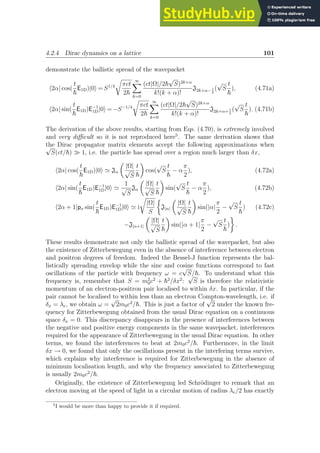
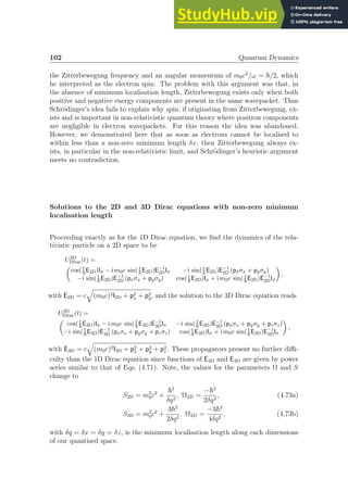
![4.3. Dynamics of Rydberg-excited Mott-insulators 103
4.3 Dynamics of Rydberg-excited Mott-insulators
Physicists like to think that all you have to do is say, these are the con-
ditions, now what happens next?
R. P. Feynman
In this final section we investigate the dynamics of systems of strongly interacting
Rydberg-excited Mott insulators using the method of walk-sums. We are interested
in determining the existence of crystalline dispositions of the Rydberg excitations
as well as coherent crystalline dispositions of the excitations, known as supersolids.
This new phase of matter, characterised by the simultaneous existence of both di-
agonal and off-diagonal long-range order, was first suggested to exist in Helium
[112, 113, 114, 115]. Recent studies have shown that supersolid phases might be ob-
tainable in optical-lattices [116, 117, 118]. In contrast to these results, the possible
dynamical creation of supersolids remains largely unexplored [119]. A system ideally
suited to study this question is that of Rydberg-excited atoms from a Mott insulator
in an optical lattice. These are formed by laser driving in the presence of strong
long-range dipole-dipole interaction. The interaction causes the excitation proba-
bility of an atom to either be inhibited (blockade) or be enhanced (antiblockade)
depending on the presence of a nearby Rydberg-excited atom. Previously quan-
tum computation and simulation schemes using similar effects have been proposed
[120, 121, 122, 123, 124]. Subsequent studies have shown that crystalline disposi-
tions of the Rydberg excitations could form the ground states of certain 1D and 2D
lattices [125, 126, 127, 128] and could also be created dynamically [129, 130, 131].
Yet these studies have not found supersolidity and have been confined to specific
parameter regimes.
In this section we explore both non coherent transient crystal phases in 1D and
3D and highly correlated supersolids in 2D lattices. In particular we show that the
lowest order of walk-sums provides simple analytical insights into small time dynam-
ics while higher orders allow us to simulate the system in strongly interacting, highly
correlated situations. In the first sub-section below, we detail the physical model
employed for the description of Rydberg excitation in Mott-insulators. We then im-
plement the method of walk-sums to calculate the mean number of Rydberg-excited
atoms throughout the lattice and their correlations. Second, we derive simple low-
order walk-sum results for these quantities and demonstrate that Rydberg-excited
1D and 3D Mott insulators evolve over short times into crystalline dispositions of the
Rydberg excitations. The third sub-section confirms these results using a walk-sum
based mean-field like approximation of the dynamics. In particular, we show that
some of the crystals can be selectively favored through the laser detuning. Finally,
relying exclusively on walk-sums, we show that a 2D Mott insulator with 6600 atoms
evolves over longer times into far from equilibrium transient supersolid states. We
characterise these states by calculating their pressure, and first, second and fourth
order correlation-functions.](https://image.slidesharecdn.com/agraphtheoreticapproachtomatrixfunctionsandquantumdynamicsphdthesis-230805203656-4458b8ad/85/A-Graph-Theoretic-Approach-To-Matrix-Functions-And-Quantum-Dynamics-PhD-Thesis-113-320.jpg)
![104 Quantum Dynamics
4.3.1 Model system and implementation of walk-sum
We consider an ensemble of atoms that are prepared in the Mott-insulating phase
with unit filling via a strong optical lattice comprising N sites. For simplicity, we
consider the lattice to be isotropic with lattice spacing L. A laser, illuminating this
lattice from the direction d = (cos φ sin θ)x + (sin φ sin θ)y + (cos θ)z where e.g. x
is the unit length vector in the x direction, drives the atoms from their ground state
|gi to a highly-excited Rydberg state |ri with principal quantum number n. We
assume that atomic transitions to other internal levels are negligible such that the
atoms are well described by two-level systems. Two Rydberg atoms at lattice sites i
and j interact via the long-range dipole-dipole interaction that is of the form [120]
Aij = (4πǫ0R3
ij)−1
µi.µj − 3R−2
ij (µi.Rij)(µj.Rij)
, (4.74)
with Rij the relative distance between atoms i and j and µi the dipole moment
of atom i. We take all the dipoles to be parallel to the laser beam orientation d,
i.e. µi = µi d with µi = kµik. Furthermore, the dipole moments of all atoms are
identical µi = µj ≡ µ and equal to µ = (3/2)n(n − 1)ea0 [132], with e the electron
charge and a0 the Bohr radius. The laser and dipole-dipole interactions we consider
are in the MHz-GHz range and induce dynamics fast compared to incoherent pro-
cesses and the motion of the atoms. These will limit the lifetime of Rydberg-excited
quantum states created by fast laser pulses to several µs but can safely be neglected
on the much shorter time scales considered here [133]. In this limit and with the
rotating-wave approximation the atoms are described by the Hamiltonian [120]
H =
X
i
n
∆Pi
−
1
2
Ω σi
x +
1
2
X
j6=i
AijPi
Pj
o
, (4.75)
with ∆ the laser detuning, Ω the Rabi-frequency, σx the Pauli matrix, Pi
= |riihri|
and, for later convenience Gi
= Ii
− Pi
= |giihgi|, the projectors onto the Rydberg
and ground states of atom i, respectively. For later convenience we also introduce
the Rydberg-radius aR as the distance between two excited atoms along direction d
such that |A(aR)| = Ω. For linear, square and cubic lattices with a lattice spacing
L, the ratio aR/L characterises the strongly and weakly interacting regimes with
aR/L 1 and aR/L . 1, respectively.
We are interested in the real time dynamics of the system governed by the Hamil-
tonian of Eq. (4.75) and in particular in the number of and correlations between Ryd-
berg excitations throughout the lattice. Thus we will concentrate our computational
efforts on calculating the Rydberg-fraction fR =
P
jhPji/N and two-excitation cor-
relation function g2(i, j) = hPi
Pj
i/hPi
ihPj
i, also known as density-density correla-
tion function. On an infinite lattice these quantities can be expressed simply in terms
of two conditional expectation values: hri/rji and hri/gji, the probabilities that atom
i be excited knowing atom j is excited and knowing that it is in its ground-state, re-
spectively. Indeed, translational symmetry implies that any atom has the same prob-
ability to be excited hPi
i = hPj
i, and therefore fR = hPi
i = hri/rjihPj
i+hri/gjihGj
i.](https://image.slidesharecdn.com/agraphtheoreticapproachtomatrixfunctionsandquantumdynamicsphdthesis-230805203656-4458b8ad/85/A-Graph-Theoretic-Approach-To-Matrix-Functions-And-Quantum-Dynamics-PhD-Thesis-114-320.jpg)
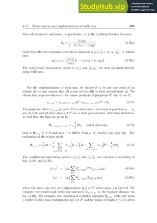
![106 Quantum Dynamics
by
Ũj←0(s) ≃
iΩ
2
M̃jM̃0 +
iΩ
2
3 X
p=1
p6=j, p6=s
M̃j(M̃0 + M̃j,p)(M̃p + M̃j)M̃0, (4.81)
where subscript 0 denotes the configuration with no excited atom. In this expression,
the factors iΩ/2 and (iΩ/2)3
come from the flips and M̃i1...in (s) = L
exp[−iHi1...in t]
.
The sum over p in Eq. (4.81) accounts for an up-spin in an intermediate configuration
of S′
that is not present in the initial and final configurations. Note that interme-
diate atomic-excitations are similar to virtual particles appearing in the Feynman
diagrams of QED. In the following section we discuss the results we obtain for fR
and g2(s, j).
4.3.2 Lowest order results
The procedure presented in the preceding section allows us to simulate the dynamics
of the system resulting from the full Hamiltonian. In order to study the dynamics
over long times t π/Ω and deeply in the strongly interacting regime L ≪ aR, we
find it necessary to take into account all walks up to length 6. Such evolution times
are required to study the development of long-range correlations in 2D lattices and
the apparition of transient supersolid states which we discuss in §4.3.4. Nevertheless,
it is also useful to dispose of low order approximations of the dynamics that are valid
over short times t . π/Ω and which can be obtained at little computational cost.
Therefore in this section we explore the lowest order walk-sum approximations for
the Rydberg fraction and density-density correlation function.
At the lowest order of walk-sum only those histories of S′
that have the minimum
possible number of jumps between the initial and final configurations are considered.
First, for hrs/gji we find according to Eqs. (4.80)
hrs/gji =
Ω2
χ2
sin
χ
2
t
2
, (4.82)
with χ2
= ∆2
+ Ω2
the generalised Rabi frequency. This result can be understood
using one-body physics. Indeed, in the case of hrs/gji, the history of S′
with the
smallest number of jump starts and ends on |gg . . . gi and has no jumps at all, i.e.
S′
is frozen from 0 to t in |gg . . . gi. During this history, atom S evolves as an
isolated 2-level atom whose transition is driven by a laser with detuning ∆ and Rabi
frequency Ω, hence Eq. (4.82). Second, in the case of hrs/rji one must consider those
final configurations of S′
where j is excited. Since all the atoms of S′
are initially in
their ground state, at least j needs to undergo the transition |gi → |ri for the final
configuration of S′
to comprise j in its Rydberg state. Thus the lowest non-zero
order is the first order, i.e. the shortest history of S′
connecting the initial and final
configurations has one jump |gg . . . gj . . . gi → |gg . . . rj . . . gi and the lowest order
approximation of hrs/rji is](https://image.slidesharecdn.com/agraphtheoreticapproachtomatrixfunctionsandquantumdynamicsphdthesis-230805203656-4458b8ad/85/A-Graph-Theoretic-Approach-To-Matrix-Functions-And-Quantum-Dynamics-PhD-Thesis-116-320.jpg)
![4.3.2 Lowest order results 107
D=W
D=0
D=-W
0.0 0.5 1.0 1.5 2.0 2.5
0.0
0.2
0.4
0.6
0.8
1.0
1.2
1.4
LaR
g
2
Hi,i+1L
D=W
D=0
D=-W
0.0 0.5 1.0 1.5 2.0 2.5
0.0
0.2
0.4
0.6
0.8
1.0
1.2
1.4
LaR
g
2
Hi,i+1L
Figure 4.8: Density-density correlation function between nearest neighbours g2(i, i+
1) on an infinite 1D lattice as a function of the lattice spacing in units of the Rydberg
radius L/aR, evaluated at the 1st order of walk-sum Eqs. (4.76b, 4.80,4.83b) (solid
blue lines), and using the Ω-expansion (dashed black lines). The time is t = π/4Ω
(left figure) and t = π/2Ω (right figure). The transition between the strongly and
weakly interacting regimes clearly occurs around L ≃ aR as expected. Parameters
d = z, n = 40 and Ω = 30MHz, which yields aR ≃ 13µm.
hrs/rji =
hgs|U†
0→jPsUj←0|gsi
hgs|U†
0→jUj←0|gsi
, (4.83a)
U1←0(t) = −i
Z t
0
e−iH1(t−t1)
H1←0e−iH0t1
dt1. (4.83b)
Evaluating these expressions present no difficulty and yields the first order result
for hrs/rji. This result is cumbersome and will not be reproduced here. Together
with Eqs. (4.76) and (4.82), this provides the first order approximation to fR and
g2(s, j). We will discuss the result for fR in the following section and for now
we concentrate on the density-density correlation function g2(s, j). We show this
quantity on Fig. 4.8 where we compare it to the prediction of the Ω-expansion
[134], denoted g2(s, j)Ω, which is a perturbative expansion of the density-density
correlation function in Ω. The differences between the two grow with time and with
the laser detuning. Indeed, for t π/Ω and/or |∆| Ω, the Ω-expansion yields
unrealistically large values for the density-density correlation function, typically in
the 103
− 104
range. This behavior is due to the Ω-expansion being valid only in
the weakly interacting regime L aR. Indeed we find that when t . π/Ω, the
Ω-expansion follows very closely
g2(s, j)Ω ≃
hrs/rji
hrs/gji
. (4.84)
From Eq.(4.76b), we see that this estimation is correct only in the weakly interacting
regime where 1 − hrs/rji + hrs/gji ≃ 1, that is hrs/rji − hrs/gji ≃ 0. In particular
this fails for L . aR and large laser detunings |∆| Ω because of strong blockade
or antiblockade effects [135, 136, 130].
The interest of the density-density correlation function lies in that it qualifies](https://image.slidesharecdn.com/agraphtheoreticapproachtomatrixfunctionsandquantumdynamicsphdthesis-230805203656-4458b8ad/85/A-Graph-Theoretic-Approach-To-Matrix-Functions-And-Quantum-Dynamics-PhD-Thesis-117-320.jpg)
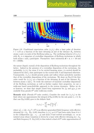
![4.3.2 Lowest order results 109
10
20 0 -10 -20
10
20
0
-10
-20
x L
y
L
g2Hs,jL
10
20 0 -10 -20
10
20
0
-10
-20
x L
g2Hs,jL
0
1
0.5
1.15
Figure 4.10: Two-body correlation-function g2(s, j) between the central atom S
(white) and any other atom j in a N ≃ 1700 atoms square lattice, one atom / pixel.
Left figure : lowest order Eq. (4.86b), right figure : converged 3rd order result,
the two results are in good agreement. Parameters θ = π/2, φ = 0, L = 2µm,
∆ = Ω = 30MHz and t = π/2Ω.
hrs/rji. Eqs. (4.76) then give very simple expressions for the Rydberg fraction and
two-excitations correlation function
fR =
(Ω2
/χ2
) sin χ
2
t
2
1 − Ω2
χ2
sj
sin
χsj
2
t
2
+ Ω2
χ2 sin χ
2
t
2 , (4.86a)
g2(s, j) =
χ2
sin
χsj
2
t
2
χ2
sj sin χ
2
t
2
h
1 −
Ω2
χ2
sj
sin
χsj
2
t
2
+
Ω2
χ2
sin
χ
2
t
2
i
. (4.86b)
We find Eq.(4.86b) to work well for small times t . π/Ω and in the weakly inter-
acting regime or in strongly blockaded situations, where the probability of finding
more than one excitation in the vicinity of S and j is small. This condition is easily
fulfilled in 1D systems where we find indeed Eq. (4.86b) to yield similar results to
the Ω-expansion [134] provided |∆| . Ω with ∆ ≤ 0. Positive detunings in the
strongly interacting regime L . aR lead to antiblockade effects which are largely
missed by the zeroth order. The zeroth order result can be a good approximation
for short times in higher dimensions as well, as shown on Fig. 4.10 where we com-
pare Eq. (4.86b) to a converged 3rd order result over a 2D square lattice. We find
however that the time spans over which zeroth order results are valid vary widely
depending on the geometry and regime considered, e.g. in 3D antiblockade effects
are inevitable and very important deep in the strongly interacting regime L ≪ aR,
where the 0th
order result fails even for very short times. Finally, we remark that
in spite of its simplicity, Eq. (4.86b) predicts a 2nd
order quantum phase transition
with critical point ∆ = Ω = 0, where g2 is non-analytic. Additionally, the minimum
distance separating two uncorrelated atoms, i.e. the correlation length, diverges
as one approaches the critical point, another signature of phase transition. This
transition was predicted in random clouds of atoms in [125] and corresponds to a](https://image.slidesharecdn.com/agraphtheoreticapproachtomatrixfunctionsandquantumdynamicsphdthesis-230805203656-4458b8ad/85/A-Graph-Theoretic-Approach-To-Matrix-Functions-And-Quantum-Dynamics-PhD-Thesis-119-320.jpg)
![110 Quantum Dynamics
change of ground state, from a crystal of excitations in the positive detuning region
to state |gg . . . gi for negative detunings. At the opposite of Eq.(4.86b), we consis-
tently find Eq. (4.86a) to be a poor approximation of fR as given by higher orders
or by the mean-field-like approach of §4.3.3. This is because the pseudo 0th
order
result Eq. (4.86a) depends explicitly on Rsj although, by translational symmetry of
the infinite lattice, it should not. That is, Eq. (4.86a) breaks an important symmetry
of the exact Eq.(4.76a).
4.3.3 Crystals of Rydberg excitations
We have seen the signature of crystals of Rydberg excitations through g2(s, j) at
order 1. To confirm the apparition of these crystals, we perform a mean-field-like
approximation of the exact Hamiltonian. This consists of simplifying the form of
the interaction with [125]
AsjPs
Pj
≃ Asj Ps
fR + Pj
fR − f2
R
g2(s, j). (4.87)
Introducing this in the Hamiltonian of Eq. (4.75), we obtain a block diagonal mean-
field Hamiltonian, each block being
Hs(t) = ∆Ps −
1
2
Ω σs
x +
X
js
hrs/rjiAsjPs, (4.88)
where we used fR g2(s, j) = hrs/rji. Using walk-sum results for hrs/rji the mean-
field-like Hamiltonian above is completely determined. We solve the resulting time-
dependent Schrödinger equation numerically and, by translational symmetry of the
infinite lattice, we obtain the Rydberg fraction as fR = hPs
i. We observe that for
t . π/Ω and L aR, the mean-field-like Rydberg fraction is nearly indistinguishable
from the first-order walk-sum result for fR. The two differ however in the strongly
interacting regime where higher orders are required to obtain similar fR from walk-
sum.
We investigate the existence of crystalline disposition of Rydberg excitations
from the mean-field-like approach by calculating fR as a function of the laser de-
tuning in the strongly interacting regime L aR. Indeed, due to the inter-atomic
interactions, we expect atoms participating in a crystal Lκ where Rydberg excita-
tions are located every κ sites to perceive this crystal with an effective detuning
of ∆eff = ∆ +
P
(j,k)∈Lκ
Ajk. When the laser detuning is such that ∆eff = 0, the
crystal is antiblockaded and the excitation probability of any atom participating in
the crystal is enhanced. Therefore if the crystal Lκ is populated, fR(∆) should peak
at ∆ = −
P
j∈Lκ
Asj. We show such a behavior of fR(∆) on Fig. (4.11) in the case
of an infinite cubic lattice.](https://image.slidesharecdn.com/agraphtheoreticapproachtomatrixfunctionsandquantumdynamicsphdthesis-230805203656-4458b8ad/85/A-Graph-Theoretic-Approach-To-Matrix-Functions-And-Quantum-Dynamics-PhD-Thesis-120-320.jpg)
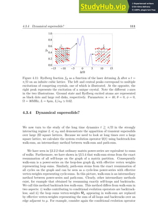
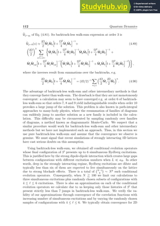
![114 Quantum Dynamics
Figure 4.12: Backtrack-less walk-sum obtained correlation-functions multiplied by
the number of pairs a) g′
1(s, j), b) g1(s, j) and c) g2(s, j) over a square lattice
with N ≈ 6600 atoms. There is one atom/pixel, S is the central one. In c),
g2(s, j) ≃ 0 except at the few sites where S and j form a free pair. d) Locations
of the dominant peaks of g4 = hPsPjPkPli/hPsihPjihPkihPli (black squares) and
g′
4 = hGsPjPkPli/hGsihPjihPkihPli (red disks) for all j, k forming free pairs with
S. Convergence indicates a precision ∼ 10−4
. Parameters : square lattice in the
xy-plane, lattice spacing L = 1.5µm, Rydberg state principal number n = 40,
Ω = 30MHz, ∆ = 0, t = 8π/Ω, laser angles θ ∼ 0.43π and φ = π/2. The system is
deeply in the strongly interacting regime aR/L ≃ 9.
effect of a time-dependent contraction of the lattice spacing L(t) on the system. The
resulting Hamiltonian H′
(t) commutes with itself at any time as well as with any
of the PiPj thus leaving fR unchanged while E(t) =
P
i,j Aij(t)hψ(t0)|PiPj|ψ(t0)i
changes only through L(t). This yields p2D = (3/2)E/A. As discussed above the
sum over hPiPji in E(t) is dominated by free pairs for which Aij = 0. We thus
find these states to have a very small pressure. Physically this is because Eq. (4.91)
is independent of the lattice spacing L. Consequently, during a contraction, atoms
forming free pairs never interact directly and the system keeps a nearly vanishing
potential energy E. We expect the small pressure to increase the lifetime of the
observed states τ ∝ p
−1/2
2D compared to states containing interacting excitations.
Indeed, in the latter case, interactions between the excitations induce center of
mass motions of the Rydberg atoms that destroy the states.
The presence of both diagonal and off-diagonal long-range order together with
a nearly vanishing quantum pressure qualifies the observed states as supersolids
[137, 138]. Their translational symmetry become apparent from 4-body correlation-
functions as shown in Fig. (4.12-d). It is important to note that these supersolid
states are far from equilibrium and do not appear in the phase diagram of the
Hamiltonian, rather they are dynamically created by the laser. The behavior of the
supersolids over very long evolution times t ≫ π/Ω remains an open question. Dur-
ing the evolution times we can simulate with walk-sum, i.e. t . 10 π/Ω, we observe
a gradual increase in the long-range correlations. This could indicate an absence of
thermalisation but the question cannot be immediately settled. Additionally, a re-
alistic simulation of the very long time dynamics of large 2D Rydberg-excited Mott
insulators will have to take into account decoherence effects, which are beyond the
scope of this work.](https://image.slidesharecdn.com/agraphtheoreticapproachtomatrixfunctionsandquantumdynamicsphdthesis-230805203656-4458b8ad/85/A-Graph-Theoretic-Approach-To-Matrix-Functions-And-Quantum-Dynamics-PhD-Thesis-124-320.jpg)

![Chapter 5
Dynamical Localisation in a
Many-Body System
Physics is mathematical not because we know so much about the physical
world, but because we know so little; it is only its mathematical properties
that we can discover.
B. Russell
In this chapter, we characterise and study dynamical localisation of a finite
interacting quantum many-body system. We present explicit bounds on the disorder
strength required for the onset of localisation of the dynamics of arbitrary ensemble
of sites of the XYZ spin-1/2 model. We obtain these results using a novel form
of the fractional moment criterion, which we establish, together with the path-sum
representation of the system resolvent. These techniques are not specific to the XYZ
model and hold in a much more general setting. We further present detailed bounds
constraining two observable quantities in the localised regime: the magnetisation of
any sublattice of the system as well as the linear magnetic response function of the
system. We confirm our results through numerical simulations.
The work of this chapter forms the basis of an article that is currently under
review for publication in Communications in Mathematical Physics and was carried
out in collaboration with Mark Mitchison and Juan Jose Mendoza-Arenas for the
TEBD simulations and with Zheng Choo for Lemma 5.6.1.
5.1 Introduction
The mathematical and physical understanding of Anderson localisation for a single
particle in a lattice with random on-site potentials has greatly progressed since it
was first recognised in 1958 [139, 140, 141]. In contrast, the theory of many-body
localisation is still in its infancy, despite the large amount of recent research focusing
on localisation in disordered many-particle systems (for example Refs. [142, 143,
144, 145, 146, 147, 148, 149, 150, 151, 152, 153]). In particular, there is still no
clear consensus on the precise definition of the many-body localised phase, with a
number of different definitions having been proposed in the recent literature (e.g.
Refs. [143, 145, 154, 149, 153, 155]). Consequently, a global picture of many-body
localisation is still lacking.
An important advance towards the conceptual understanding of the problem
was the introduction of the notion of localisation in the quantum configuration or
Fock space [156], which has emerged as a powerful framework for understanding
117](https://image.slidesharecdn.com/agraphtheoreticapproachtomatrixfunctionsandquantumdynamicsphdthesis-230805203656-4458b8ad/85/A-Graph-Theoretic-Approach-To-Matrix-Functions-And-Quantum-Dynamics-PhD-Thesis-127-320.jpg)
![118 Dynamical Localisation in a Many-Body System
many-body localisation [142, 143, 149, 155]. Configuration-space localisation has
also proved useful in understanding the absence of thermalisation in integrable sys-
tems [157] and glassy dynamics in strongly interacting systems [158]. Following
these developments, we treat the evolution of the many-body quantum state as that
of a single fictitious particle moving in an exponentially large configuration space.
This viewpoint leads us quite naturally to define many-body dynamical localisa-
tion as Anderson localisation of this effective one-particle problem. Furthermore, it
facilitates a non-perturbative, mathematically rigorous treatment.
Rigorous mathematical results concerning localisation in interacting many-body
systems have been established in [154] and [159]. However, the critical disorder in-
ducing a many-body localisation transition as predicted by these studies is difficult
to ascertain and the physical consequences of the localisation remain, in part, unex-
plored.The contribution of the present work to the study of many-body localisation
is thus three-fold. First we provide an explicit bound for the critical amount of
disorder necessary for localisation to occur. Second, we make concrete predictions
of experimental signatures of the localisation by providing bounds for two physically
observable quantities in the localised regime: the magnetisation of any finite ensem-
ble of sites immersed in the system as well as the linear magnetic response function.
We confirm our predictions with Time Evolving Block Decimation (TEBD) simula-
tions of a 1D system. Third, our approach to many-body localisation differs from
existing approaches [154] and [159]. While we do use a form of fractional moment
criterion as a mathematical signature of localisation, we rely on the path-sums rep-
resentation of the Green’s functions associated to any sublattice of the full system
to prove that this criterion is met for a finite amount of disorder. The path-sums
approach employed here facilitates the manipulation and systematic representation
of matrix resolvents and Green’s functions. Thus, we hope that it will ultimately
contribute to the proof of localisation in infinite interacting many-body systems,
which remains elusive.
The chapter is organised as follows. In §5.2 we present the model system and
general mathematical strategy we employ. For the sake of concreteness we focus
on the particular case of a finite, interacting spin-1
2
system described by the XYZ-
Hamiltonian. This section culminates in a criterion characterising the localised
regime. In §5.3 we begin with bounds for the onset of dynamical localisation in
one-body systems as well as bounds for the onset of localisation of functions of
random matrices. In §5.3.2 we give similar results in the many-body setting. We
then provide precise constraints for the magnetisation of arbitrary sublattices of
the system as well as the correlations between spins at sites of the sublattice in
the localised regime. The bound on the latter quantity is shown to imply a bound
on the linear magnetic response function to magnetic perturbations, which we find
to be vanishingly small deep in the localised regime. The proofs of all technical
results are given in section §5.4-§5.8. Section §5.5 contains the proof of the main
result concerning the onset of localisation and a brief presentation of the path-sums
approach. In §5.6 we gather the proofs of technical lemmas necessary to the proof
presented in §5.5. Finally, in §5.7 and §5.8 we derive the results concerning the](https://image.slidesharecdn.com/agraphtheoreticapproachtomatrixfunctionsandquantumdynamicsphdthesis-230805203656-4458b8ad/85/A-Graph-Theoretic-Approach-To-Matrix-Functions-And-Quantum-Dynamics-PhD-Thesis-128-320.jpg)
![5.2. Model system and approach 119
magnetisation and correlations in the localised regime.
5.2 Model system and approach
5.2.1 Model system
The XYZ-Hamiltonian
We consider a lattice L of N spin-1/2 particles governed by the XYZ-Hamiltonian,
which represents one of the simplest models of strongly-interacting many-body sys-
tems. The Hamiltonian reads
H =
X
i
Biσz
i +
X
hiji
Jxσx
i σx
j + Jyσy
i σy
j + ∆σz
i σz
j , (5.1)
where Jx, Jy and ∆ are real and parametrise the spin-spin interactions, and
P
hiji
denotes a sum over nearest neighbours. The {Bi}i∈[1,N] variables are local magnetic
fields which we assume to be independent and identically distributed (iid) random
variables taken from a Gaussian distribution with standard deviation σB. For con-
venience, we choose the basis states of the Hilbert space to be configurations of
spins along the direction of the magnetic fields, e.g. for a two spin-1/2 system this
is {|↑↑i, |↑↓i, |↓↑i, |↓↓i}, where ↑ and ↓ designate the situations where the spin is
aligned and antialigned with the magnetic fields, respectively.
For Jx 6= Jy, the XYZ-Hamiltonian does not conserve the total number of up and
down spins present at any time in the system. Since we can add the sum of all the
random magnetic fields
P
i Bi to the Hamiltonian without affecting the dynamics,
an up spin is effectively equivalent to a particle seeing a random onsite potential
2Bi at site i, while a down spin always sees 0 onsite potential, being effectively
equivalent to the absence of a particle. In this sense, the XYZ Hamiltonian does
not conserve the number of particles present in the system. At the opposite, when
Jx = Jy, the number of up- and down-spins present in the system is conserved by
H. We call this specific situation the XXZ regime.
Mathematical description
We consider the total system described by the XYZ Hamiltonian (5.1), denoted by
S, as comprising two parts S and S′
. We shall use a partial basis of the configu-
ration space of S that specifies only the state of S′
. From hereon we designate the
configurations available to S and S′
by Roman and Greek letters, respectively.
Mathematically this procedure corresponds to working with a tensor product
partition of the Hamiltonian into smaller matrices, see Chapter 3. Recall that these
small matrices, denoted Hω←α, are submatrices of H of size 2|S|
× 2|S|
with |S| the
number of sites in S and fulfill the characteristic relation of tensor product partitions
|ωihα| ⊗ Hω←α = Pω ⊗ IS
. H . Pα ⊗ IS
, (5.2a)](https://image.slidesharecdn.com/agraphtheoreticapproachtomatrixfunctionsandquantumdynamicsphdthesis-230805203656-4458b8ad/85/A-Graph-Theoretic-Approach-To-Matrix-Functions-And-Quantum-Dynamics-PhD-Thesis-129-320.jpg)
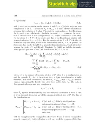
![5.2.2 Dynamics of the system equivalent particle 121
which is bounded as follows kHω←αk ≤ nL(J2
x +J2
y )1/2
:= nLJ , with nL the maximum
number of neighbours that any site of S′
has on the lattice L. On Euclidean lattices
L ≡ Zd
, this is 2d
.
5.2.2 Dynamics of the system equivalent particle
Our goal is to establish dynamical localisation of S′
regardless of the state of S. In
many-body situations, it is useful to consider localisation of the system directly in
its configuration space rather than on the physical lattice [143, 149, 154]. As long as
the system is finite, the configuration space associated to any partition S = S ∪ S′
of the system is a discrete graph GS,S′ , which we construct as follows:
i) For each configuration α available to S′
, we draw a vertex vα.
ii) If Hω←α 6= 0, we draw an edge (αω) from vertex vα to vertex vω.
iii) To each edge (αω), we associate the weight Hω←α.
Finally, we define d(α, ω) the distance between two configurations of the system as
the length of the shortest walk on GS,S′ from vertex vα to vertex vω.
The configuration graph gives an alternative picture of the system dynamics. For
the choice S = ∅, S′
= S the statics and flips are the matrix entries of the Hamilto-
nian Hω←α = (H)ωα and the dynamics in real space is equivalent to that of a single
particle in the configuration space, which we call the System Equivalent Particle
(SEP), undergoing a continuous time quantum random walk on G∅,S. Furthermore,
in the XXZ regime where Jx = Jy, if there is initially single up-spin in a sea of
down-spins (or the opposite), the configuration graph G∅,S is simply the real-space
lattice and the SEP represents this single up-spin.
For general partitions S = S ∪ S′
, S can be interpreted as the internal degree of
freedom of the SEP, while its trajectory on the graph GS,S′ represents the evolution
of S′
. When S′
is in configuration α, the SEP is on site vα and feels the random
potential Yα, which we then call the configuration potential at α. Depending on the
amount of disorder present in the various configuration potentials, the SEP may be
dynamically localised, which corresponds to many-body localisation of S′
, regardless
of the state of S.
5.2.3 Criterion for many-body localisation
In analogy with the case of a single particle on a lattice [141], the natural signature
of SEP dynamical localisation is simply the absence of diffusion of the SEP on GS,S′ .
This is expressed rigorously using the same tensor product partition that we used
for the Hamiltonian but this time for the evolution operator PI(H)e−iHt
, where PI is
the projector onto the eigensubspace of H with energy in bounded interval I. The
elements of this partition fulfill the characteristic relation
|ωihα| ⊗
PI(H)e−iHt
ω←α
= Pω ⊗ IS
. PI(H)e−iHt
. Pα ⊗ IS
, (5.6a)](https://image.slidesharecdn.com/agraphtheoreticapproachtomatrixfunctionsandquantumdynamicsphdthesis-230805203656-4458b8ad/85/A-Graph-Theoretic-Approach-To-Matrix-Functions-And-Quantum-Dynamics-PhD-Thesis-131-320.jpg)
![122 Dynamical Localisation in a Many-Body System
or equivalently
PI(H)e−iHt
ω←α
= hω| ⊗ IS
. PI(H)e−iHt
. |αi ⊗ IS
. (5.6b)
For convenience, we say that (PI(H)e−iHt
)ω←α is a flip of the evolution operator when
ω 6= α and, otherwise, a static of the evolution operator. In this formalism, localisa-
tion of the SEP on the configuration graph GS,S′ is characterised by an exponential
bound on the norm of the flips of the evolution operator (~ = 1)
E
sup
t∈R
PI(H)e−iHt
ω←α
≤ Ce−d(α,ω)/ζ
, (5.7a)
or equivalently
E
sup
t∈R
hω| ⊗ IS
PI(H)e−iHt
|αi ⊗ IS
≤ Ce−d(α,ω)/ζ
. (5.7b)
In these expressions E[.] is the expectation with respect to all the random variables,
supt∈R is the supremum over time, C ∞, ζ 0 and k.k is the 2-norm. Note, for
the choice S = ∅, S′
= S, Eq. (5.7) reduces to an exponential bound on off-diagonal
matrix elements of the evolution operator.
By construction, the criterion of Eqs. (5.7) is a natural extension of the criterion
for dynamical localisation of isolated particles. Furthermore, we show below that
the criterion is met for a finite amount of disorder in a finite interacting many-
body system described by the XYZ-Hamiltonian of Eq. (5.1) and that once verified,
Eqs. (5.7) lead to constraints on the magnetisation of S′
, the correlations between
its sites and the linear magnetic response function.
Before we progress, three remarks are in order. First, for technical reasons,
we only consider finite energy intervals I. We note however that for any realistic
finite system this is not constraining since there must be a finite energy interval
containing all possible spectra of the random XYZ model1
. Second, from now on
we restrict ourselves to sublattices S′
comprising only non-adjacent sites. This is
not a fundamental requirement of our approach, but it facilitates the mathematical
proofs. The case of adjacent sites is discussed in Remark 5.3.9, p. 127 below. Third,
since we consider a finite system with exclusively discrete degrees of freedom, the
spectrum of H is discrete.
By construction, the criterion of Eq. (5.7b) is a natural extension of the crite-
rion for dynamical localisation of isolated particles. Furthermore, we show below
that the criterion is met for a finite amount of disorder in a finite interacting many-
body system described by the XXZ-Hamiltonian of Eq. (5.1) and that once verified,
Eq. (5.7b) leads to strong constraints on the magnetisation of S′
and on the corre-
lations between its sites.
1
We do not assume nor use this in the mathematical proofs.](https://image.slidesharecdn.com/agraphtheoreticapproachtomatrixfunctionsandquantumdynamicsphdthesis-230805203656-4458b8ad/85/A-Graph-Theoretic-Approach-To-Matrix-Functions-And-Quantum-Dynamics-PhD-Thesis-132-320.jpg)
![5.3. Dynamical localisation 123
5.3 Dynamical localisation
In this section we present the main results of the present chapter. For the sake of
clarity, we only sketch here the outline of the proofs and defer all the proofs to §5.4
and §5.5. In §5.3.1, we begin with bounds for the onset of dynamical localisation
in one-body systems as well as bounds for the onset of localisation of functions of
random matrices. In §5.3.2 we give bounds for the onset of dynamical localisation
in a many-body system and in §5.3.3-5.3.4 we describe observable signatures of this
localisation.
5.3.1 One-body localisation and localisation of matrix func-
tions
We begin by studying the simplest situation: that of single up-spin in a sea of down-
spins (or the opposite), in the XXZ regime. In this case, the problem is effectively
one-body since in the XXZ regime, the Hamiltonian conserves the total number
of up- and down-spins present in the system at any time. One-body dynamical
localisation is now a well understood phenomenon and Theorem 5.3.1 presented in
this section is already known [160, 161, 141]. For the sake of completeness and since
its derivation uses a simple form of path-sum, we include it in this chapter.
Theorem 5.3.1 (One-body dynamical localisation). Consider a single particle evolv-
ing on Zδ
according to the Hamiltonian of Eq. (5.1). Let I be an interval of energy
with finite Lebesgue measure |I|. Let a and b be two points of Zδ
and d the distance
between them. Then for all 0 s 1,
E
h
sup
t∈R
ha|PIe−iHt
|bi
i
≤ C e− d
(2−s)ζ , (5.8a)
where
ζ−1
= ln
h 1 − s
2δ − 1
σB
√
2π
2|J|
si
0 for σB
2δ − 1
1 − s
1/s 2|J|
√
2π
, (5.8b)
C =
1
2π
2|I|
1
2−s
kρks
∞
1 − s
2δ
2δ − 1
1
1 − e−1/ζ
, (5.8c)
with kρk∞ = 1/(σB
√
2π).
The path-sum based proof of this proposition is presented in §5.4. We also obtain
a more general mathematical result concerning the average exponential decay of
uniformly bounded functions of certain finite random matrices:
Theorem 5.3.2 (Localisation of matrix functions). . Let {Yα} be an ensemble of
independent random variables with probability distributions ρα Hölder continuous of
order 1 and define kρk∞ = maxα kραk. Let M ∈ Cn×n
be a normal matrix, R its
spectral radius and RM(z) = (zI−M)−1
its resolvent. If there exists a partition {Mαω}
of M such that all statics are of the form Mαα = YαI+M̃αα with M̃αα a deterministic](https://image.slidesharecdn.com/agraphtheoreticapproachtomatrixfunctionsandquantumdynamicsphdthesis-230805203656-4458b8ad/85/A-Graph-Theoretic-Approach-To-Matrix-Functions-And-Quantum-Dynamics-PhD-Thesis-133-320.jpg)
![124 Dynamical Localisation in a Many-Body System
matrix, then for all 0 s 1 and any bounded function f(z) analytic on a region
containing all the possible spectra Sp(M), we have
E
h
RM(z)
αω
s
i
≤
X
ℓ≥d(α,ω)
|ΠG;αω|(ℓ)
Ωℓs
αω
(1 − s)ℓ+1
(2kρk∞)sℓ+s
, (5.9a)
where G is the graph of the partition, Ωαω = maxα,ω kMαωk and E[.] represents
the expectation with respect to all random variables. Furthermore, if Ωs
αω (1 −
s)(2kρk∞)−1
, then the expected weight of a fully dressed prime walk decays exponen-
tially with its length. In this situation,
E
h
RM(z)
αω
s
i
≤
kρks
∞
1 − s
2
1 − e−1/ζ
e−
d(α,ω)
ζ , (5.9b)
E
h
sup
t∈R
f(M)αω
i
≤
1
2π
kfk∞(2R)
1
2−s
kρks
∞
1 − s
2
1 − e−1/ζ
e−
d(α,ω)
(2−s)ζ , (5.9c)
where
ζ−1
= ln
h 1 − s
λG kρks
∞Ωs
αω
i
0, (5.9d)
with λG the largest eigenvalue of G.
Remark 5.3.1 (Structure of the random matrices). The theorem is to be under-
stood as a statement regarding random matrices with fixed structure. In other words,
the emplacement of the zero entries of M does not vary and only the non-zero entries
are allowed to be random. This fixes the graph G and the distance d(α, ω) between
any two vertices is well defined.
Remark 5.3.2 (Sparsity of M). Although the theorem holds even when M is full,
in this situation the theorem becomes trivial since maxα,ω{d(α, ω)} = 1.
Remark 5.3.3 (Off-diagonal disorder). The theorem still holds if each flip is also
a function of a random variable. In this situation, let Yαω be the random variable
upon which Mαω depends. Then, if for all flips the expectation EYαω
kMαωk
exists,
the theorem remains valid upon replacing Ωαω by maxα,ω EYαω
kMαωk
.
Remark 5.3.4 (Correlated random variables). Let (α1η2 · · · αj · · · αℓ) be a prime
walk on G. Then the Theorem holds in the situation where the Yα are correlated
upon replacing kρkℓ
∞ by
Qℓ
j=1 kραj|k∞, where kραj|k∞ is the infinity norm of the
conditional probability distribution of Yαj
knowing Yαj+1
, · · · , Yαℓ
.
5.3.2 Many-body localisation
A major difficulty in the study of many-body localisation as compared to one-body
localisation lies in that the effective amount of disorder present in the system grows
only logarithmically with the size of the relevant space GS,S′ . Indeed, since there
are only |S′
| random B-fields affecting the sites of S′
, there are only |S′
| linearly](https://image.slidesharecdn.com/agraphtheoreticapproachtomatrixfunctionsandquantumdynamicsphdthesis-230805203656-4458b8ad/85/A-Graph-Theoretic-Approach-To-Matrix-Functions-And-Quantum-Dynamics-PhD-Thesis-134-320.jpg)
![5.3.2 Many-body localisation 125
independent configuration potentials. In the same time S′
can adopt up to 2|S′|
con-
figurations. Thus, the total amount of disorder affecting the SEP is very small as
compared to the size of the space on which it evolves. Furthermore, this disorder is
also highly correlated, as the configuration potentials are linearly dependent. These
observations explain why the proof of localisation for many-body systems is much
more involved than its one-body counterpart and leads to much larger bounds on
the minimum amount of disorder required for localisation to happen.
Outline of our approach:
We obtain a bound on the disorder strength required for the many-body localisation
criterion Eq. (5.7a) to be met as follows:
1) We relate Eq. (5.7a) to a novel form of fractional moment criterion. More
precisely, we consider generalised Green’s functions which evolve the SEP on its
configuration space. These are matrices dictating the evolution of S′
regardless
of that of S. They arise from a tensor product partition of the system resolvent
(zI−H)−1
. We show that if fractional powers of the 2-norm of these generalised
Green’s functions are exponentially bounded, then Eq. (5.7a) is satisfied.
2) We express generalised Green’s functions non-perturbatively using the method
of path-sums, which represents the generalised Green’s functions as a super-
position of simple paths undergone by the SEP on its configuration space.
Simple paths are walks forbidden from visiting any vertex more than once.
On Euclidean lattices they are known as self-avoiding walks.
3) Using path-sums representations, we directly obtain an upper-bound on the
required fractional norms. No induction on the number of particles is required,
in contrast to Refs. [154] and [159].
These steps finally yield the main theorem of the present chapter (see §5.5 for de-
tails):
Theorem 5.3.3 (Many-body dynamical localisation in an interacting system). Con-
sider an ensemble of particles evolving on a finite lattice L comprising N sites ac-
cording to the XYZ-Hamiltonian of Eq. (5.1). Let S′
an ensemble of non-adjacent
lattice sites and I be an interval of energy with finite Lebesgue measure |I|. Then
for any 0 s 1 and any 2−|S′|
s1 1,
E
sup
t∈R
PI(H)e−iHt
ω←α
≤ C(ω, α) e
−
(s1−s)
s1(2−s)
d(α,ω)
ζ
, (5.10a)](https://image.slidesharecdn.com/agraphtheoreticapproachtomatrixfunctionsandquantumdynamicsphdthesis-230805203656-4458b8ad/85/A-Graph-Theoretic-Approach-To-Matrix-Functions-And-Quantum-Dynamics-PhD-Thesis-135-320.jpg)
![126 Dynamical Localisation in a Many-Body System
where
C(ω, α) =
1
2π
2|I|
1
2−s
c[s1]
s
s1
2−|S′|s
Ds
(σB
√
2π)s
× (5.10b)
1
s|S′|
Φ e−1/ζ
, 1, d(α, ω) + 1 − s−1
s1−s
s1
,
ζ−1
= s log
σB
√
2π
DnLJ |S′|1/s
, (5.10c)
where ζ is the localisation length and
ζ 0 if and only if σB σmin
B = DnLJ |S′
|1/s
/
√
2π. (5.10d)
In these expressions, J = (J2
x +J2
y )1/2
, nL is the maximum number of neighbours that
any site of S′
has on L, D = 2N
, c[s1] = 41−s1
ks1
/(1−s1) where k is a finite universal
constant and Φ is the Hurwitz-Lerch zeta-function, which decays algebraically with
d(α, ω) when d(α, ω) s−1
− 1.
Remark 5.3.5 (Meaning of the bound). Because we partition the system into two
subsystems S and S′
, we emphasise that the meaning of the above bound is dif-
ferent from what is usually understood from such bounds. If Eq. (5.10a) holds for
some disorder σB and sublattice S′
comprising |S′
| non-adjacent sites, then the dy-
namic of any and hence all sublattices comprising |S′
| non-adjacent sites is localised,
regardless of the dynamics of the rest of the system.
Remark 5.3.6 (Dependency on the system size). The bound we obtain on the
critical amount of disorder required for the onset of localisation scales exponentially
with the system size N. This is unsurprising in view of the fact that the XYZ
Hamiltonian does not conserve the number of particles in the system. For this
reason, adding a single site to the lattice doubles the number of configurations
available to the system.
Remark 5.3.7 (Dependency on the system partition). In the situation where the
Hamiltonian is partitioned into its matrix elements, i.e. the flips and statics are
the entries of the Hamiltonian Hω←α = (H)ωα, we have S = ∅, S′
= S and thus
|S′
| = |S| = N. This degrades both the bound on the critical disorder σmin
B and the
localisation length ζ linearly with the system size. It is therefore beneficial to use
partitions with small |S′
| values.
Remark 5.3.8 (Dependency on the interaction strength along z). The bound ob-
tained above for the critical amount of disorder does not depend on the interaction
parameter ∆, but rather holds for any ∆. This is because of a crucial step of our
proof, where we determine a bound for the norm of a generalised Green’s functions
independently of the details of the self-energy. By the same token, we lose infor-
mation about any influence the interaction strength ∆ might have on the onset of
localisation. Thus, our approach does not permit us to study the influence of ∆.](https://image.slidesharecdn.com/agraphtheoreticapproachtomatrixfunctionsandquantumdynamicsphdthesis-230805203656-4458b8ad/85/A-Graph-Theoretic-Approach-To-Matrix-Functions-And-Quantum-Dynamics-PhD-Thesis-136-320.jpg)
![5.3.3 Localisation of sublattice magnetisation 127
We could partially circumvent this problem by treating the deterministic interaction
term in configuration α as a realisation of a random variable ˜
∆α whose probability
distribution can be evaluated from the Hamiltonian. Then one would take expecta-
tions with respect to a new random configuration potential Ỹα = Yα + ˜
∆α and the
strength ∆ of the interaction would play a role similar to the variance of the random
B-fields.
Remark 5.3.9 (Dependency on the lattice). The theorem holds regardless of the
dimension and details of the physical lattice. This is because we require S′
to
comprise only non-adjacent sites. In this situation, the configuration graph GS,S′
must be an |S′
|-hypercube H|S′| or a subgraph of it, regardless of the physical lattice.
Indeed, H|S′| connects all configurations of S′
differing by one spin flip. Thus if
the configuration graph is not H|S′| or a subgraph of it, then there is at least one
transition allowed between two configurations of S′
differing by two spin flips. This
corresponds to two non-adjacent spins flipping at the same time, which is not allowed
by the Hamiltonian. This approach leads to simpler results when deriving observable
signatures of the localised regime, see §5.3.3, §5.3.4 and Appendices 5.7 and 5.8. Our
results can nonetheless be extended so as to hold in situations where S′
comprises
adjacent sites. For example, if the physical lattice is Zd
, d ≥ 1, then the bound on
the critical disorder becomes σmin
B = D2d
J d1/s
|S′
|1/s
/(2
√
2π).
Remark 5.3.10 (Extension to other Hamiltonians). While we present Theorem
5.3.3 explicitly in the case of the XYZ-Hamiltonian, we do so for the sake of con-
creteness. The arguments developed in the proof of the theorem do not make use of
the specifics of the XYZ-Hamiltonian, so that the theorem can easily be extended
other Hamiltonians and other probability distributions ρ for the random magnetic
fields2
, as considered in Ref. [154].
Remark 5.3.11 (Use of the 2-norm). Theorem 5.3.3 is stated in terms of the 2-norm
which might seem to obscure the physical meaning of the bound Eq. (5.10a). Indeed
physical quantities of interest such as the system magnetisation and correlations
functions are most naturally expressed in terms of the Frobenius norm. Nonetheless
we show explicitly in the next section that Theorem 5.3.3 implies constraints on
such physical quantities, as would be expected if the theorem involved the Frobenius
norm.
5.3.3 Localisation of sublattice magnetisation
In this section and the next we discuss observable consequences of the criterion for
many-body localisation Eq. (5.7a). Although the bound for the onset of many-body
localisation presented in Theorem 5.3.3 holds for any finite ensemble of non-adjacent
sites S′
, there is a particular choice of sites for S′
that leads to a simple structured
configuration graph, allowing for easier interpretations of the consequences of SEP
dynamical localisation.
2
So long as ρ remains Hölder continuous.](https://image.slidesharecdn.com/agraphtheoreticapproachtomatrixfunctionsandquantumdynamicsphdthesis-230805203656-4458b8ad/85/A-Graph-Theoretic-Approach-To-Matrix-Functions-And-Quantum-Dynamics-PhD-Thesis-137-320.jpg)
![128 Dynamical Localisation in a Many-Body System
Suppose that S′
consists of a set of sites that are well separated in real space.
In this case, the surrounding sites belonging to S effectively act as a spin bath
with which the sites of S′
can freely exchange spin excitations. Clearly, S will act
more effectively as a bath in higher dimensions, when each site of the lattice has
more nearest neighbours. A key consequence of this choice is that the number of
up-spins in S′
can vary, even in the XXZ regime Jx = Jy where the total number
of up spins in the entire system is conserved. Thus, in this situation and regardless
of the values of Jx and Jy, every one of the 2|S′|
configurations available to S′
is
accessible. Furthermore, each configuration of S′
is connected to exactly |S′
| other
configurations, because each spin within S′
is free to flip its state when Jx 6= Jy, or, in
the XXZ regime, by virtue of its contact with the spins of S. These considerations
uniquely specify the configuration graph of S′
as the |S′
|-hypercube. Then the
dynamics of the SEP is that of a particle undergoing a continuous-time quantum
random walk on the hypercube, perceiving highly correlated random potentials at
the various sites.
Now an important consequence of the structure of the hypercube is that the
distance d(α, ω) between any two configurations α and ω available to S′
is at least
equal to the difference between the number of up-spins in the two configurations
d(α, ω) ≥ |nα −nω|, with nα the number of up-spins in S′
when it is in configuration
α. Thus SEP dynamical localisation as per our criterion Eq. (5.7a) immediately
implies localisation in the number of up-spins in the sublattice
E
sup
t∈R
PI(H)e−iHt
n′←n
≤ Ce−|n−n′|/ζ
, (5.11a)
or equivalently
E
h
sup
t∈R
k hn′
| ⊗ IS
PI(H)e−iHt
|ni ⊗ IS
k
i
≤ Ce−|n−n′|/ζ
, (5.11b)
where |ni and |n′
i represent any superposition of configurations of S′
with exactly
n and n′
up-spins, respectively.
This yields an observable signature of the many-body localisation of the system:
the magnetisation of any sublattice is constrained within an interval centered on its
value at time t = 0. More precisely, let N↑
S′ (t) and N↓
S′ (t) be the number of up-
and down-spins in the sublattice S′
at time t, respectively. We define the disorder-
averaged normalised magnetisation as M(t) = E
N↑
S′ (t) − N↓
S′ (t)
/|S′
|, with E[.] the
expectation with respect to all random magnetic fields. In Appendix 5.7 we show
that this quantity is bounded at any time as follows
1 − n↓
(ζ) ≤ M(t) ≤ n↑
(ζ) − 1, (5.12)
with n↑
(ζ) and n↓
(ζ) two time-independent quantities depending on the localisation](https://image.slidesharecdn.com/agraphtheoreticapproachtomatrixfunctionsandquantumdynamicsphdthesis-230805203656-4458b8ad/85/A-Graph-Theoretic-Approach-To-Matrix-Functions-And-Quantum-Dynamics-PhD-Thesis-138-320.jpg)
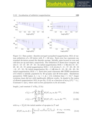
![130 Dynamical Localisation in a Many-Body System
•
•
•
•
•
•
•
•
•
0.3 0.4 0.5 0.6 0.7 0.8
0.4
0.6
0.8
1
Log@ΣBÈS'ÈD-1
Mt •
•
•
•
•
•
•
•
•
0.3 0.4 0.5 0.6 0.7
-0.3
0
0.3
0.7
1
Log@ΣBÈS'ÈD-1
Mt
•
•
•
•
•
•
•
•
•
•
0.4 0.6 0.8 1.0
0.5
0.7
0.9
1
Log@ΣBÈS'ÈD-1
Mt •
•
•
•
•
•
•
•
•
•
0.4 0.6 0.8 1.0
0.4
0.6
0.8
1
Log@ΣBÈS'ÈD-1
Mt
aL bL
cL dL
Figure 5.2: Same simulations as in Figure 5.1, but here fitting the values of C and
ζ independently for each figure. The TEBD results are consistent with localisation
of the system in its configuration space.
In the strongly localised regime, the bound Eq. (5.12) becomes
lim
ζ→0
1 − n↓
(ζ) = lim
ζ→0
n↑
(ζ) − 1 = M(0), (5.15)
that is the sublattice magnetisation is constrained around its initial value, as ex-
pected. On Figures (5.1) and (5.2) we compare the bounds of Eq. (5.12) with TEBD
simulations of a half-filled 1D lattice of 60 sites in the XXZ regime. Our implemen-
tation of the TEBD algorithm is based on the open-source Tensor Network Theory
(TNT) library [162]. We use C and ζ as free parameters to fit the simulation results
with our theoretical predictions. This means that we do not use their values as pre-
dicted by Theorem 5.3.3. This is because we could only simulate disorder strengths
σB which are below the bound σmin
B obtained in the theorem. In Fig. (5.1) we deter-
mine the values of C and ζ so as to fit the magnetisations of all observed sublattices
at once. Our result are in good agreement with the simulated magnetisations, which
demonstrates that the behaviour of this physical quantity is well captured by our
bound Eq. (5.12). In particular, the simulations show that the sublattice magneti-
sation is strongly constrained around its initial value deep in the localised regime, as
predicted by our theoretical bounds. In Fig. 5.2, the values of C and ζ are fitted for
each sublattice separately. The excellent agreement between theory and simulation
here shows that the overall dependency of the simulated magnetisation with the
disorder is very well captured by our bounds.
These results demonstrate the validity of our criterion, which quantitatively pre-
dicts a physically observable signature of many-body localisation.](https://image.slidesharecdn.com/agraphtheoreticapproachtomatrixfunctionsandquantumdynamicsphdthesis-230805203656-4458b8ad/85/A-Graph-Theoretic-Approach-To-Matrix-Functions-And-Quantum-Dynamics-PhD-Thesis-140-320.jpg)
![5.3.4 Localisation of sublattice correlations and magnetic susceptibility 131
0.00 0.05 0.10 0.15 0.20
0
15
30
-15
-30
ΖÈS'È
i
Χ
i,
j
HtL
0 0.06 0.12
0
-0.5
-1
ΖÈS'È
Τ
i,
j
HtL
Figure 5.3: Bounds on the disorder-averaged magnetic linear response iχi,j(t) in the
localised regime, as a function of the localisation length ζ. The shaded region is the
region allowed by the bound Eq. (5.21) We consider here a sublattice S′
comprising
|S′
| = 10 sites. Initially, the sublattice is in a configuration α with |α| = 3 up spins
and i and j are up and down in α, respectively. In inset: bound on the disorder
averaged correlation function τi,j(t), initially τi,j(0) = −1. The shaded region is the
region allowed by the bounds Eqs. (5.18).
5.3.4 Localisation of sublattice correlations and magnetic
susceptibility
Similarly to the sublattice magnetisation presented above, we prove in Appendix 5.8
that once the criterion for many-body dynamical localisation Eq. (5.7a) is fulfilled,
then the correlations between any two sites of the sublattice S′
will be localised
around their initial value. The correlations at time t between two sites i and j of S′
that we consider are given by
τi,j(t) = E
Tr[PI(H) σi
z(t) PI(H) σj
z ρS]
, (5.16)
where E[.] is the expectation with respect to all random magnetic fields, ρS is the
initial density matrix of the entire system S and σi
z(t) = eiHt
σi
ze−iHt
. The quan-
tity τt(i, j) is of interest because it relates to the disorder-averaged linear magnetic
response function χi,j(t). More precisely we have
χi,j(t) = −i E
h[σi
z(t), σj
z(0)]i
= −i τi,j(t) − τj,i(−t)
, (5.17)
which determines the response of the magnetisation at site i to a time-dependent
magnetic field applied at site j [163].
In the situation where S′
is initially in a single configuration α and is dynamically
localised as per our criterion Eq. (5.7a), we obtain the following bounds for the
sublattice correlations](https://image.slidesharecdn.com/agraphtheoreticapproachtomatrixfunctionsandquantumdynamicsphdthesis-230805203656-4458b8ad/85/A-Graph-Theoretic-Approach-To-Matrix-Functions-And-Quantum-Dynamics-PhD-Thesis-141-320.jpg)
![5.4. Proofs of the one-body results 133
again, our criterion for many-body dynamical localisation implies strong constraints
on an observable physical quantity.
5.4 Proofs of the one-body results
Consider the situation where a single up-spin lives in a sea of down-spins (or the
opposite) in the XXZ regime. In this situation we choose the most natural (and only
physically meaningful) partition S = ∅, S′
= S. Mathematically, this corresponds to
partitioning the Hamiltonian into its usual matrix elements. Choosing this partition,
the configuration graph is identifiable to the physical lattice and a configuration of S′
simply specifies the position of the unique up-spin. Consequently, the configuration
potentials Yα are of the form 2Bα −B with Bα the random magnetic field felt by the
up-spin at site α and B the total sum of all random magnetic fields. This quantity
is an overall energy shift to the Hamiltonian and can be removed without affecting
the results3
. Finally, we note that the generalised Green’s functions reduce to the
usual Green’s functions.
Consider two points a and b of Zδ
and let d be their distance. The starting
point of the proof of one-body localisation in δ-dimensions is the following criterion,
discovered by Aizenman and Molchanov [164],
(
∃C ∞, ζ 0, 0 s 1 with
E
h
G(a, b; z)
s
i
≤ Ce−d/ζ
,
=⇒
(
∃C′
∞, ζ′
0 with
E
h
supt∈R ha|PIe−iHt
|bi
i
≤ C′
e−d/ζ′
,
(5.24)
where we may use C′
= 1
2π
2|I|
1
2−s
C, as we prove in a more general setting in §5.6.1.
Relying on this criterion, we prove in this section that the fractional moments of
the system Green’s functions G(a, b; z)
s
are, on average, exponentially bounded.
5.4.1 One-dimensional chain
We first consider a 1D chain of down-spins, denoted L. Initially, a single up-spin is
present on site a. Let b be another site of L located at a distance d from a. Since
there is always only a single simple path between any two points of L, the path-sum
representation of the system Green’s function G(a, b; z) yields
E
|G(a, b; z)|s
= |2J|ds
E
d
Y
j=0
GLj (aj, aj; z)
s
#
,
≤ |2J|ds
E
d
Y
j=0
GLj (aj, aj; z)
s
#
, (5.25)
3
Calculations with and without B yield the same bound for the onset of localisation.](https://image.slidesharecdn.com/agraphtheoreticapproachtomatrixfunctionsandquantumdynamicsphdthesis-230805203656-4458b8ad/85/A-Graph-Theoretic-Approach-To-Matrix-Functions-And-Quantum-Dynamics-PhD-Thesis-143-320.jpg)
![134 Dynamical Localisation in a Many-Body System
with a0 ≡ a, ad ≡ b, Lj
≡ L{a0, · · · , aj−1}, E[.] the expectation with respect to the
random magnetic fields and we used Haj+1←aj
= 2J. We progress by transforming
the expectation of Eq. (5.25) into nested conditional expectations:
E
|G(a, b; z)|s
= |2J|ds
(5.26)
E{B}[a,b]
EBad
|
· · · EBa1 |
EBa0 |
h d
Y
j=0
GLj (aj, aj; z)
s
i
· · ·
##
.
In this expression, EBaj |[.] is a short hand notation for the conditional expectation
with respect to the magnetic field Baj
at site aj knowing Baj+1
, · · · , Bad
and all
magnetic fields affecting sites outside of the interval [a, b]. Finally, E{B}[a,b][.] is the
expectation with respect to the magnetic fields affecting sites outside of the interval
[a, b].
At this point it is essential to recall that the product over Green’s functions rep-
resents a simple path. Thus the magnetic field Bak
appearing in GLj≤k (aj≤k, aj≤k; z)
cannot appear in any of the subsequent Green’s functions GLjk (ajk, ajk; z) since
once traversed by the simple path, site ak has been removed form the lattice L. In
particular, the only Green’s function that can depend on Ba0 is GL(a0, a0; z). Then,
EBa0 |
h d
Y
j=0
GLj (aj, aj; z)
s
i
=
d
Y
j=1
GLj (aj, aj; z)
s
EBa0 |
h
GL(a0, a0; z)
s
i
, (5.27)
Furthermore, the dependency of GL(a0, a0; z) on Ba0 is very simple: indeed by virtue
of the path-sum representation of matrix inverses, we have
GL(a0, a0; z) =
z − 2Ba0 − Ha0 − Σ0
−1
, (5.28)
with Ha0 is the deterministic part of the potential felt by the spin at site a0 and Σ0
the sum of all cycles off a0 on L0
. In this context however, it is known as the self-
energy. It is noteworthy that the self-energy being a sum of cycles on L0
≡ L{a0},
it does not depend on Ba0 and, by construction, neither does z − Ha0 . Therefore,
the dependency of |GL(a0, a0; z)|s
on Ba0 is of the form |2Ba0 + M|−s
, with M ∈ C.
Thanks to these observations and using the result of Proposition 5.5.2 (see p. 141),
the conditional expectation of Eq. (5.27) is upper bounded by
EBa0 |
h
GL(a0, a0; z)
s
i
≤
kρks
∞
1 − s
. (5.29)
where kρk∞ = 1/(σB
√
2π) is the infinity-norm of the probability distribution ρ of
the random magnetic fields, with σB its variance.
We then repeat the above procedure for all the subsequent conditional expec-
tations, always observing that |GLj (aj, aj; z)|s
is of the form |Baj
+ M|−s
for some](https://image.slidesharecdn.com/agraphtheoreticapproachtomatrixfunctionsandquantumdynamicsphdthesis-230805203656-4458b8ad/85/A-Graph-Theoretic-Approach-To-Matrix-Functions-And-Quantum-Dynamics-PhD-Thesis-144-320.jpg)
![5.4.2 δ 1 dimensional lattices 135
M ∈ C which does not depend on Baj
. Thus we obtain
E
|G(a, b; z)|s
≤ |2J|ds
E{B}[a,b]
1
(1 − s)(σB
√
2π)s
d+1
#
,
=
kρks
∞
1 − s
×
(2|J|)ds
(1 − s)d
1
(σB
√
2π)ds
. (5.30)
This exhibits exponential decay with d as soon as σB 2|J|/
√
2π(1 − s)1/s
for
some 0 s 1.
5.4.2 δ 1 dimensional lattices
The only difference between the δ 1 and the δ = 1 dimensional cases is that when
the physical lattice is more than one dimensional, there exists more than one simple
path of length ℓ ≥ d between any two vertices of the lattice located at distance d
from each other. The path-sum representation of the Green’s function is then
E
|G(a, b; z)|s
= E
X
ℓ≥d
X
ΠLδ; ab; ℓ
(2J)ℓ
ℓ
Y
j=0
GLj (aj, aj; z)
s
, (5.31)
with ΠLδ; ab; ℓ the ensemble of simple-paths of length ℓ from a to b on Lδ
. Remarking
that for any ensemble of complex numbers {cj} and 0 s 1, |
P
j cj|s
≤
P
j |cj|s
,
the above becomes
E
|G(a, b; z)|s
≤
X
ℓ≥d
X
ΠLδ; ab; ℓ
|2J|ℓs
E
ℓ
Y
j=0
GLj (aj, aj; z)
s
#
. (5.32)
Each element of the sum can now be treated with the technique presented in the 1
dimensional case. Since furthermore on L(δ) ≡ Zδ
the number of simple paths of
length ℓ 0 is clearly upper bounded by 2δ(2δ − 1)ℓ−1
, we obtain
E
h
|GL(δ)(a, b; z)|s
i
≤
kρks
∞
1 − s
∞
X
ℓ=d
2δ(2δ − 1)ℓ−1
(2|J|)ℓs
(1 − s)ℓ(σB
√
2π)ℓs
, (5.33)](https://image.slidesharecdn.com/agraphtheoreticapproachtomatrixfunctionsandquantumdynamicsphdthesis-230805203656-4458b8ad/85/A-Graph-Theoretic-Approach-To-Matrix-Functions-And-Quantum-Dynamics-PhD-Thesis-145-320.jpg)
![136 Dynamical Localisation in a Many-Body System
The above series converges when σB (2δ − 1)/(1 − s)
1/s
× 2|J|/
√
2π, in which
case
E
h
sup
t∈R
ha|PIe−iHt
|bi
i
≤ C e− d
(2−s)ζ , (5.34)
ζ−1
= ln
h 1 − s
2δ − 1
σB
√
2π
2|J|
si
0 for σB
2δ − 1
1 − s
1/s 2|J|
√
2π
,
C =
1
2π
2|I|
1
2−s
kρks
∞
1 − s
2δ
2δ − 1
1
1 − e−1/ζ
. (5.35)
This establishes Proposition 5.3.1.
◮ We prove Theorem 5.3.2.
Proof. The demonstration of the theorem is entirely identical to the proof of one-
body localisation on δ ≥ 1 lattices, with the exception that the constant C′
of
Eq. (5.4) has an additional kfk∞ factor, i.e. C′
= 1
2π
2|I|
1
2−s
kfk∞C as can be seen
from the derivation of Proposition 5.5.1 below. We omit the details.
5.5 Proofs of the many-body results
5.5.1 A generalised fractional moment criterion
As we have seen in §5.2.2 and §5.2.3, localisation of the many-body dynamics is
equivalent to the dynamical localisation of the SEP on its configuration space. This
observation led to the following signature of many-body localisation Eq. (5.7b)
E
h
sup
t∈R
hω| ⊗ IS
PI(H)e−iHt
|αi ⊗ IS
i
≤ Ce−d(α,ω)/ζ
. (5.36)
In order to demonstrate that there exists a finite value of the variance σB of the
random magnetic fields such that Eq. (5.36) is satisfied, we use a generalisation of
the fractional moment criterion originally developed by Aizenman and Molchanov
in the one-body setting [164, 165]. This criterion can be summarised as follows. Let
a and b be two points of a lattice, then
(
∃C ∞, ζ 0, 0 s 1 with
E
h
G(a, b; z)
s
i
≤ Ce−d/ζ
,
=⇒
(
∃C′
∞, ζ′
0 such that
E
h
supt∈R ha|PIe−iHt
|bi
i
≤ C′
e−d/ζ′
.
where G(a, b; z) is the Green’s function evaluated between points a and b. For
our purpose it is necessary to extend this criterion to arbitrary system partitions
S = S∪S′
. In particular, one must extend the notion of Green’s function between two
points of a lattice to that of Green’s functions between two configurations accessible
to S′
.
This is easily achieved using a tensor-product partition of the system resolvent
RH(z) = zI − H
−1
. In continuity with existing conventions regarding the Green’s](https://image.slidesharecdn.com/agraphtheoreticapproachtomatrixfunctionsandquantumdynamicsphdthesis-230805203656-4458b8ad/85/A-Graph-Theoretic-Approach-To-Matrix-Functions-And-Quantum-Dynamics-PhD-Thesis-146-320.jpg)
![5.5.2 Bounding the norms of generalised Green’s functions 137
functions, we denote the elements of this partition
GGS,S′ (ω, α; z) := RH(z)
ω←α
, (5.37)
and call them generalised Green’s functions. These are 2|S|
× 2|S|
submatrices of the
system resolvent RH(z). As required of a tensor-product partition of the resolvent,
the generalised Green’s functions fulfill the characteristic relation
|ωihα| ⊗ GGS,S′ (ω, α; z) = Pω ⊗ IS
. RH(z) . Pα ⊗ IS
, (5.38a)
with Pα = |αihα|. Equivalently,
GGS,S′ (ω, α; z) = hω| ⊗ IS
. RH(z) . |αi ⊗ IS
. (5.38b)
Using generalised Green’s functions, Aizenman’s fractional moment criterion can be
extended to arbitrary system partitions:
Lemma 5.5.1 (Fractional moment criterion for arbitrary system partitions). Let
S = S ∪ S′
be a system partition, GS,S′ the graph associated to it and d(α, ω) the
distance between vertices vα and vω on GS,S′ . If there exists C ∞ and ζ ∞ such
that, for 0 s 1,
E
h
GGS,S′ ω, α; z
s
i
Ce−d(α, ω)/ζ
, (5.39)
then
E
sup
t∈R
PI(H)e−iHt
ω←α
≤
1
2π
2|I|
1
2−s
Ce−
d(α,ω)
(2−s)ζ , (5.40)
where |I| is the Lebesgue measure of I.
To preserve the flow of the argument, we defer the proof of this result to Appendix
5.6.1. Thanks to Lemma 5.5.1 above, we may focus our efforts on bounding fractional
norms of the generalised Green’s functions. We achieve this using their path-sums
representation.
5.5.2 Bounding the norms of generalised Green’s functions
Following the result of Lemma 5.5.1, we are left with the task of proving that there
exists an amount of disorder σB such that the fractional norms of generalised Green’s
functions are exponentially bounded, i.e.
E
h
GGS,S′ ω, α; z
s
i
≤ Ce−d(α,ω)/ζ
, (5.41)
with s ∈ (0, 1), C ∞ and most importantly 0 ζ ∞.
In the spirit of the proof for the one-body situation [141], we bound the expec-
tation of the fractional moments of the generalised Green’s functions using their](https://image.slidesharecdn.com/agraphtheoreticapproachtomatrixfunctionsandquantumdynamicsphdthesis-230805203656-4458b8ad/85/A-Graph-Theoretic-Approach-To-Matrix-Functions-And-Quantum-Dynamics-PhD-Thesis-147-320.jpg)
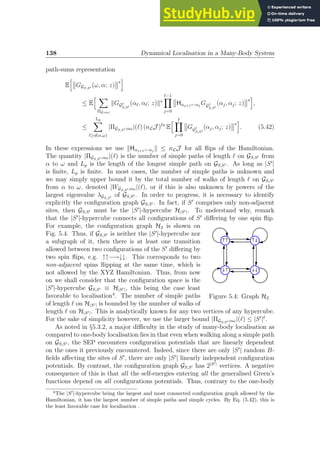
![5.5.2 Bounding the norms of generalised Green’s functions 139
case, the generalised Green’s functions have a complicated dependency on the con-
figuration potentials. This dependency is analytically accessible for sufficiently small
S′
, e.g. |S′
| = 1 − 6, yet analytical calculations of the required expectations remain
very difficult as we shall see below.
Another consequence of the linear dependency between the configuration po-
tentials is that we cannot distribute the conditional expectations in the product
of generalised Green’s functions as is possible in the one-body case. This fur-
ther complicates the calculation of the required expectation along a simple path
E
h Qℓ
j=0 GGj
S,S′
(αj, αj; z)
s
i
. In order to recover simpler expressions, we note that
the expectation above involves the product measure d̺{Bj}j /
∈S′
Q|S′|
j=1 d̺Yαj
, with ̺Yαj
the cumulative distribution function of Yαj
. Therefore, we can upper bound the
expectation of a product of norms of generalised Green’s functions by a product of
expectations on using the generalised Hölder inequality [166]. This leads to
E
h ℓ
Y
j=0
GGj
S,S′
(αj, αj; z)
s
i
≤
ℓ
Y
j=0
E
h
GGj
S,S′
(αj, αj; z)
qjs
i1/qj
, (5.43)
with
Pℓ
j=0 q−1
j = 1. We will see below that the above can only be bounded if qjs 1
for all j. Using qj = ℓ + 1 for all j we thus need s 1/(ℓ + 1) to guarantee the
existence of the above expectations. Since the graph GS,S′ is a subgraph of H|S′|,
the longest simple path has length at most ℓ = Lp ≤ 2|S′|
and s 1/(2|S′|
+ 1)
is sufficient to guarantee existence of all expectations. We will see later that this
requirement on s can be waived using a technical result from Ref. [154].
We now turn to bounding expectations of individual generalised Green’s func-
tions. Using conditional expectations we have
E
h
GGj
S,S′
(αj, αj; z)
sj
i
= E{Bj}j /
∈S′ , {Yαi }i6=j
EYαj |
h
GGj
S,S′
(αj, αj; z)
sj
i
, (5.44)
with sj = qjs and EYαj |[.] is the expectation with respect to Yαj
knowing the value
of |S′
| − 1 linearly independent configuration potentials affecting S′
, here denoted
{Yαi
}i6=j, as well as all magnetic fields affecting sites outside of the sublattice S′
.
As noted earlier, thanks to path-sum, for sufficiently small |S′
| (typically less
than 6) the exact dependency of a generalised Green’s functions on a certain config-
uration potential is explicitly accessible. Yet, this dependency is still too complicated
to be used to bound the expectation of the Green’s function with respect to this
configuration potential. To see this, let us consider again the simple example where
S′
comprises only two sites, denoted 1 and 2. In this situation the configuration
graph of |S′
| is the square H2 and the configurations available to S′
are ↑↑, ↑↓, ↓↑
and ↓↓, see Fig. (5.4). The corresponding configuration potentials are Y↑↑ = B1 +B2,](https://image.slidesharecdn.com/agraphtheoreticapproachtomatrixfunctionsandquantumdynamicsphdthesis-230805203656-4458b8ad/85/A-Graph-Theoretic-Approach-To-Matrix-Functions-And-Quantum-Dynamics-PhD-Thesis-149-320.jpg)
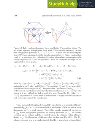
![5.5.2 Bounding the norms of generalised Green’s functions 141
obtain the generalised Green’s function of the collapsed vertex as
GGj
S,S′ (Yαj )(vYαj
, vYαj
; z) =
h
zI − Yαj
I − ΣYvαj
i−1
, (5.46)
where ΣvYαj
is the self-energy associated to the ensemble of configurations which are
linearly dependent on Yαj
, i.e. it is the sum of all cycles off vYαj
on Gj
S,S′ (Yαj
){vYαj
}.
Since all vertices whose configuration potential is linearly dependent on Yαj
have
been merged to form vYαj
, none of the remaining vertices of Gj
S,S′ (Yαj
){vYαj
} depend
on Yαj
. Consequently, ΣvYαj
is independent of Yαj
. Furthermore, GGj
S,S′
(αj, αj; z)
is a submatrix of GGj
S,S′ (Yαj )(vYαj
, vYαj
; z): more precisely it is the submatrix cor-
responding to S′
being in configuration αj. From these observations we deduce
kGGj
S,S′
(αj, αj; z)ksj
≤ GGj
S,S′ (Yαj )(vYαj
, vYαj
; z)
sj
, (5.47)
and therefore
EYαj |
h
kGj
GS,S′
(αj, αj; z)ksj
i
≤ EYαj|
h
GGj
S,S′ (Yαj )(vYαj
, vYαj
; z)
sj
i
. (5.48)
The right hand side of the above is bounded thanks to the following lemma, whose
proof we defer to Appendix 5.6.2:
Lemma 5.5.2. Let Y be a normally distributed random variable with density func-
tion ρ. Let A ∈ Cn×n
be a normal matrix. Then the following bound holds for any
0 s 1,
EY
h
[Y I + A]−1 s
i
≤
(2n)s
1 − s
kρks
∞, (5.49)
where k.k is the 2-norm and k.k∞ the infinity norm.
Using the lemma and on assuming that sj 1, we obtain
EYαj|
h
GGj
S,S′ (Yαj )(vYαj
, vYαj
; z)
sj
i
≤
(2Dj)sj
1 − sj
kρYαj|
ksj
∞. (5.50)
The quantity Dj is the dimension of GGj
S,S′ (Yαj )(vYαj
, vYαj
; z) or, in other terms, Dj
is the rank of the perturbation associated with modifications of Yαj
. We bound Dj
on noting that: i) each vertex of GS,S′ is associated with a vector space of dimension
2|S|
; ii) at most half of the vertices of GS,S′ are linearly dependent on any given
configuration potential. From these observations it follows that Dj ≤ 2|S|
×2|S′|
/2 :=
D/2. Finally, ρYαj|
is the probability distribution of configuration potential Yαj
knowing the value of |S′
| − 1 linearly independent configuration potentials affecting
S′
as well as all magnetic fields affecting sites outside of the sublattice S′
. We
show in §5.6.4 that this distribution is normal and its variance is at least σB. Taken
together, Eqs. (5.48) and (5.50) thus yield the following bound concerning individual](https://image.slidesharecdn.com/agraphtheoreticapproachtomatrixfunctionsandquantumdynamicsphdthesis-230805203656-4458b8ad/85/A-Graph-Theoretic-Approach-To-Matrix-Functions-And-Quantum-Dynamics-PhD-Thesis-151-320.jpg)
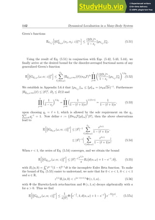
![5.5.2 Bounding the norms of generalised Green’s functions 143
In this expression, we have defined
ζ−1
= s log
σB
√
2π
DnLJ |S′|1/s
, (5.57b)
i.e. r = e−1/ζ
. In particular we have,
r 1 ⇐⇒ ζ 0 ⇐⇒ σB DnLJ |S′
|1/s
/
√
2π. (5.57c)
At this point, the requirement s 1/(2|S′|
+ 1) 2−|S′|
, which we used in the proof,
clearly seems to heavily degrade the condition on σB for the onset of localisation:
indeed s 2−|S′|
⇒ σB ≥ |S′
|1/s
≥ |S′
|2|S′|
is extremely large, even for moderate
|S′
|. We circumvent this difficulty by adapting a result of Ref. [154] to our situation:
Lemma 5.5.3 (Based on Aizenman and Warzel [154]). If there exists smax 1 such
that for all s, 0 s smax,
E
h
GGS,S′ (ω, α; z)
s
i
Ce−d(α,ω)/ζ
, (5.58)
then for all s ∈ (0, 1) we have
E
h
kGGS,S′ (ω, α; z)ks
i
≤ c[s1]s/s1
2|S|s
(σB
√
2π)s
C
s1−s
s1 e
−
(s1−s)
s1
d(α,ω)
ζ
, (5.59)
with smax s1 1 and c[s1] = 41−s1
ks1
/(1 − s1) with k a finite universal constant.
We call this result the extension lemma. For the sake of clarity we defer its proof
to Appendix 5.6.3. Using the extension lemma, we may extend the exponential
bound from 0 s 1/(2|S′|
+ 1) to 0 s 1. We obtain, for all 0 s 1,
E
h
GGS,S′ (ω, α; z)
s
i
≤ c[s1]
s
s1
2−|S′|s
Ds
(σB
√
2π)s
× (5.60)
1
s|S′|
Φ e−1/ζ
, 1, d(α, ω) + 1 − s−1
s1−s
s1
e
−
(s1−s)
s1
d(α,ω)
ζ
,
where we used 2|S|
= D × 2−|S′|
and the Hurwitz-Lerch zeta-function decays al-
gebraically with d(α, ω) when d(α, ω) s−1
− 1. The results of Eqs. (5.57, 5.60)
together with Lemma 5.5.1 establish Theorem 5.3.3.
Remark 5.5.1 (Wegner estimate and dissipative operators). Instead of using Lemma
5.5.2 to upper bound EYαj|
h
GGj
S,S′ (Yαj )(vYαj
, vYαj
; z)
sj
i
as we did in Eq. (5.50), we
may use two alternative arguments:
1) First, we may use the celebrated Wegner estimate for multi-particle systems
[167]. The Wegner estimate provides the spectral density of H which in turn
relates to the spectral density of ΣYvαj
. This permits an alternative calculation](https://image.slidesharecdn.com/agraphtheoreticapproachtomatrixfunctionsandquantumdynamicsphdthesis-230805203656-4458b8ad/85/A-Graph-Theoretic-Approach-To-Matrix-Functions-And-Quantum-Dynamics-PhD-Thesis-153-320.jpg)
![144 Dynamical Localisation in a Many-Body System
of an upper bound for the expectation and the end result in only a factor of 2
larger than that obtained by Lemma 5.5.2.
2) The second approach consist in noting that for z ∈ C+
, ΣYvαj
being Hermitian,
zI − ΣYvαj
is dissipative [168, 169]. This allows to bound the expectation
using arguments from [154, 170]. The bound is then extended to the entire
complex plane (using conjugation and analytic continuation) and leads to a
result similar to that obtained from Lemma 5.5.2.
These observations indicate that there is not much room for improvement of the
bound on EYαj|
h
GGj
S,S′ (Yαj )(vYαj
, vYαj
; z)
sj
i
. Rather, work aiming at improving the
overall bound for the onset of localisation should focus on bounding the expectation
of an individual generalised Green’s function from its explicit form as in Eq. (5.45),
without recurring to Y -collapses.
5.6 Technical results
In this section we regroup four technical results: 1) we prove Lemma 5.5.1 re-
lating exponential bounds on fractional norms of generalised Green’s functions to
dynamical localisation; 2) we prove Lemma 5.5.2, which provides an upper bound
on expectations of the form EY
kY I+Aks
; 3) we prove the extension Lemma 5.5.3;
and 4) we study the marginal and joint distributions of the configuration potentials.
5.6.1 Generalised fractional moment criterion
In this section we establish Lemma 5.5.1, which we restate here for convenience.
Lemma 5.5.1. Let S = S ∪S′
be a system partition, GS,S′ the graph associated to it
and d(α, ω) the distance between vertices vα and vω on GS,S′ . If there exists C ∞
and ζ ∞ such that
E
h
GGS,S′ ω, α; z
s
i
Ce−d(α, ω)/ζ
, (5.61)
then for 0 s 1,
E
h
sup
t∈R
hω| ⊗ IS
PI(H)e−iHt
|αi ⊗ IS
i
≤
1
2π
2|I|
1
2−s
Ce−
d(α,ω)
(2−s)ζ , (5.62)
where |I| is the Lebesgue measure of I.
Proof. To prove the lemma, we first use Cauchy’s integral relation for the matrix](https://image.slidesharecdn.com/agraphtheoreticapproachtomatrixfunctionsandquantumdynamicsphdthesis-230805203656-4458b8ad/85/A-Graph-Theoretic-Approach-To-Matrix-Functions-And-Quantum-Dynamics-PhD-Thesis-154-320.jpg)
![5.6.1 Generalised fractional moment criterion 145
exponential [51] to relate the exponential of the Hamiltonian with its resolvent
hω| ⊗ IS
PI(H)e−iHt
|αi ⊗ IS
= hω| ⊗ IS
1
2πi
I
γI
e−izt
RH(z)dz |αi ⊗ IS
, (5.63)
with γI a contour enclosing all the eigenvalues λ ∈ Sp(H)∩I, with Sp(H) the discrete
spectrum of H, and only these. Using a line integral along the contour γI yields the
upper bound
sup
t∈R
hω| ⊗ IS
PI(H)e−iHt
|αi ⊗ IS
≤
1
2π
Z
I
GGS,S′ ω, α; γI(x)
dγI, (5.64)
where dγI = γ′
I(x)dx and we used ke−izt
k∞ = 1 for z ∈ R 5
. More generally, for
uniformly bounded functions f(z) we would have kfk∞. In order for the fractional
moments to appear, we use Hölder’s inequality with 1 = s a+2(1−a), a = 1/(2−s)
and s ∈ (0, 1) [161]. This gives
Z
I
GGS,S′ ω, α; γI(x)
dγI ≤
Z
I
GGS,S′ ω, α; γI(x)
2
dγI
1−a
×
Z
I
GGS,S′ ω, α; γI(x)
s
dγI
a
. (5.65)
Now we show that the first term of the right hand side is upper bounded by 1.
To this end, we note that Sp(H) is discrete and the eigenvalues have almost surely
multiplicity one [161, 171]. Furthermore, H is Hermitian and thus if the domain is
finite, the spectral theorem indicates that for all λ ∈ Sp(H),
lim
ε↓0
−iε RH(λ + iε) = Pλ, (5.66)
with Pλ = |ϕλihϕλ| the projector onto the eigenstate corresponding to eigenvalue λ.
Therefore,
Z
I
GGS,S′ ω, α; γI(x)
2
dγI =
X
λ∈Sp(H)∩I
khω|Pλ |αik2
=
X
λ∈Sp(H)∩I
khω|Pλ |αihα|Pλ |ωik,
=
X
λ∈Sp(H)∩I
khω|ϕλihϕλ|αihα|ϕλihϕλ|ωik, (5.67)
where we used kMk2
= kMM†
k and |αi and |ωi are short hand notations for |αi⊗IS
and |ωi ⊗ IS, respectively. Now we remark that hϕλ|αihα|ϕλi is a positive real
number which we denote |hϕλ|αi|2
, and similarly hω|ϕλihϕλ|ωi ≡ |hϕλ|ωi|2
∈ R+
.
5
We need only consider z ∈ R as all the poles of the resolvent are on the real line so that the
contour can be brought arbitrarily close to it.](https://image.slidesharecdn.com/agraphtheoreticapproachtomatrixfunctionsandquantumdynamicsphdthesis-230805203656-4458b8ad/85/A-Graph-Theoretic-Approach-To-Matrix-Functions-And-Quantum-Dynamics-PhD-Thesis-155-320.jpg)
![146 Dynamical Localisation in a Many-Body System
Thus
X
λ∈Sp(H)∩I
khω|ϕλihϕλ|αihα|ϕλihϕλ|ωik ≤
X
λ∈Sp(H)∩I
|hϕλ|ωi|2
X
λ′∈Sp(H)∩I
|hϕλ′ |αi|2
,
≤ 1. (5.68)
Inserting this result in Eq. (5.65) and then in Eq. (5.64) yields the bound
sup
t∈R
hω|PI(H)e−iHt
|αi ≤
1
2π
Z
I
GGS,S′ ω, α; γI(x)
s
dγI
1
2−s
. (5.69)
The remaining steps are entirely similar to those exposed in [161] and [171]. Taking
the expectation values on both sides, we note that 1/(2 − s) 1 and Hölder’s
inequality yields E
|f|1/(2−s)
≤ E
|f|
1/(2−s)
. Now Fubini’s theorem gives
E
h
sup
t∈R
hω|PI(H)e−iHt
|αi
i
≤
1
2π
Z
I
E
h
GGS,S′ ω, α; γI(x)
s
i
dγI
1
2−s
. (5.70)
To progress further, we recall the M-L inequality, also called estimation lemma:
Proposition 5.6.1 (M-L inequality [172]). Let f be a complex valued function,
continuous on a contour γ and such that |f(z)| is bounded for all z ∈ γ. Then we
have Z
γ
f(z)dz ≤ ℓ(γ) max
z∈γ
|f(z)|, (5.71)
where ℓ(γ) is the length of the contour γ.
Returning to our proof, we note that if the fractional moments of the Green’s
function are bounded by an exponential, e.g. Ce−d(α,ω)/ζ
, the M-L inequality implies
E
h
sup
t∈R
hω|PI(H)e−iHt
|αi
i
≤ CI Ce−
d(α,ω)
(2−s)ζ , (5.72)
where CI = (2π)−1
2|I|
1
2−s
since 2|I| is the length of the smallest contour enclosing
all poles within I, where |I| the Lebesgue measure of I. This result extends the
fractional moment criterion of Aizenman and Molchanov to arbitrary partitions of
the system.
5.6.2 Bounding the expectation of a fractional norm
In this section we establish Lemma 5.5.2, which we restate here for convenience.
Lemma 2. Let Y be a normally distributed random variable with distribution func-
tion ρ. Let A ∈ Cn×n
be a normal matrix. Then the following bound holds for any](https://image.slidesharecdn.com/agraphtheoreticapproachtomatrixfunctionsandquantumdynamicsphdthesis-230805203656-4458b8ad/85/A-Graph-Theoretic-Approach-To-Matrix-Functions-And-Quantum-Dynamics-PhD-Thesis-156-320.jpg)
![5.6.2 Bounding the expectation of a fractional norm 147
0 s 1,
EY
h
[Y I + A]−1 s
i
≤
(2n)s
1 − s
kρks
∞, (5.73)
where k.k is the 2-norm.
Proof. The lemma follows from the layer-cake integral for the expectation [154].
Since A is normal and finite, there exist a unitary matrix U and diagonal matrix D
such that Y I + A = U(Y I + D)U†
. Now let Sp(A) be the spectrum of A and suppose
Y is fixed. Then
[Y I + A]−1
= max
λ∈Sp(A)
|Y + λ|−1
,
=
min
λ∈Sp(A)
|Y + λ|
−1
. (5.74)
Let 1[x] be the indicator function, which equals 1 if assertion x is true and 0 other-
wise. Then the expectation is upper bounded as follows
EY
h
[Y I + A]−1 s
i
=
Z ∞
−∞
[Y I + A]−1 s
d̺,
=
Z ∞
−∞
Z k[Y I+A]−1ks
0
1dt d̺,
=
Z ∞
−∞
Z ∞
0
1
h
[Y I + A]−1 s
t
i
dt d̺, (5.75)
where ̺ is the cumulative distribution function. By Fubini’s theorem and on using
Eq. (5.74) this is
EY
h
[Y I + A]−1 s
i
=
Z ∞
0
Z ∞
−∞
1
h
min
λ∈Sp(A)
|Y + λ| t−1/s
i
d̺ dt,
=
Z ∞
0
min
1,
Z ∞
−∞
1
h
min
λ∈Sp(A)
|Y + λ| t−1/s
i
d̺
dt. (5.76)
Now let Ii = [ai, ai+1], 0 ≤ i ≤ n − 1 be n intervals such that minλ∈Sp(A) |Y + λ| =
|Y + λi| for all Y ∈ Ii. Then
Z ∞
−∞
1
h
min
λ∈Sp(A)
|Y + λ| t−1/s
i
d̺ =
n
X
i=0
Z ai+1
ai
1
|Y + λi| t−1/s
d̺,
≤
n
X
i=0
Z ∞
−∞
1
|Y + λi| t−1/s
d̺,
=
n
X
i=0
̺ |Y + λi| t−1/s
,
≤ 2nkρk∞t−1/s
, (5.77)](https://image.slidesharecdn.com/agraphtheoreticapproachtomatrixfunctionsandquantumdynamicsphdthesis-230805203656-4458b8ad/85/A-Graph-Theoretic-Approach-To-Matrix-Functions-And-Quantum-Dynamics-PhD-Thesis-157-320.jpg)
![148 Dynamical Localisation in a Many-Body System
where, by virtue of the fact that ̺ is Hölder continuous6
, for any interval [a, b],
̺([a, b]) ≤ |a − b| K with K = supa, b ̺([a, b])/|a − b| ≤ 2kρk∞. The last step of
Eq. (5.77) is a rather crude upper bound which may be refined if more is known
about the spectrum of M. Inserting this result in Eq. (5.76) gives
EY
h
[Y I + A]−1 s
i
≤
Z ∞
0
min
1, 2nkρk∞t−1/s
dt,
=
Z m
0
1dt + 2nkρk∞
Z ∞
m
t−1/s
dt,
=
ns
1 − s
2s
kρks
∞. (5.78)
We obtain the last line on choosing the m that minimises the bound.
5.6.3 Proof of the extension lemma
In this section we prove the extension Lemma 5.5.3, which we restate here for con-
venience.
Lemma 5.5.3. (Extension lemma, based on Aizenman and Warzel [154])
If there exists smax 1 such that for all s, 0 s smax,
E
h
GGS,S′ (ω, α; z)
s
i
Ce−d(α,ω)/ζ
, (5.79)
then for all τ ∈ (0, 1) we have
E
h
kGGS,S′ (ω, α; z)kτ
i
≤ c[s1]τ/s1
2|S|τ
kρkτ
∞C
s1−τ
s1 e
−
(s1−τ)d(α,ω)
s1ζ
, (5.80)
with smax s1 1.
Proof. Let 0 s2 smax τ s1 1. Then since τ = s1(τ − s2)/(s1 − s2) +
s2(s1 − τ)/(s1 − s2), it follows that
E
h
kGGS,S′ (ω, α; z)kτ
i
(5.81)
= E
h
kGGS,S′ (ω, α; z)k
s1
τ−s2
s1−s2 kGGS,S′ (ω, α; z)k
s2
s1−τ
s1−s2
i
.
We use Hölder’s inequality to separate the above expectation into a product involv-
ing two expectations. Let q1 = (s1 − s2)/(τ − s2) and q2 = (s1 − s2)/(s1 − τ) and
6
We consider only on the case where ρ is Hölder continuous of order 1, which is the case of
the normal distribution. The proof extends well to Hölder continuous distributions of higher order
[161].](https://image.slidesharecdn.com/agraphtheoreticapproachtomatrixfunctionsandquantumdynamicsphdthesis-230805203656-4458b8ad/85/A-Graph-Theoretic-Approach-To-Matrix-Functions-And-Quantum-Dynamics-PhD-Thesis-158-320.jpg)
![5.6.4 Conditional distribution of the configuration potentials 149
remark that q−1
1 + q−1
2 = 1. Thus
E
h
kGGS,S′ (ω, α; z)kτ
i
≤ E
h
kGGS,S′ (ω, α; z)k
q1s1
τ−s2
s1−s2
i1/q1
×
E
h
kGGS,S′ (ω, α; z)k
q2s2
s1−τ
s1−s2
i1/q2
,
= E
h
kGGS,S′ (ω, α; z)ks1
i τ−s2
s1−s2
×
E
h
kGGS,S′ (ω, α; z)ks2
i s1−τ
s1−s2
. (5.82)
Now E
kGGS,S′ (ω, α; z)ks2
≤ Ce−d(α,ω)/ζ
is exponentially bounded since s2 smax.
Furthermore, E
kGGS,S′ (ω, α; z)ks1
is bounded as well. This follows from Theorem
2.1 of Ref. [154], based on results of Ref. [170]. These results give
kGGS,S′ (ω, α; z)ks1
≤ c[s1] 2|S|
s1
kρks1
∞ (5.83)
with c[s1] = 41−s1
ks1
/(1 − s1) and k a finite universal constant. Then,
E
h
kGGS,S′ (ω, α; z)kτ
i
≤
c[s1]2|S|s1
kρks1
∞
τ−s2
s1−s2
C
s1−τ
s1−s2 e
−
(s1−τ)d(α,ω)
ζ(s1−s2)
. (5.84)
Since we may choose s2 to be arbitrarily small, we obtain for all 0 τ 1,
E
h
kGGS,S′ (ω, α; z)kτ
i
≤ c[s1]τ/s1
2|S|τ
kρkτ
∞C
s1−τ
s1 e
−
(s1−τ)d(α,ω)
s1ζ
. (5.85)
This establishes the lemma.
5.6.4 Conditional distribution of the configuration poten-
tials
In this section we study the marginal and joint distribution of the configuration
potentials.
We begin our study by determining the covariance between any two configuration
potentials. To this end, we first introduce some notation. Let B = (B1, · · · , B|S′|) be
the vector of the random B-fields at the sites comprised in S′
. The {Bi}i∈S′ are iid
normal random variables with variance Var(Bi) = σ2
B. Let vα = (v
(α)
1 , v
(α)
2 , · · · , v
(α)
|S′|)
be the vector of coefficients a
(α)
i = ±1 such that
Yα = vα . B =
|S′|
X
i=1
v
(α)
i Bi, (5.86)
i.e. v
(α)
i = 1 when the spin at site i is up along z in the configuration α of S′](https://image.slidesharecdn.com/agraphtheoreticapproachtomatrixfunctionsandquantumdynamicsphdthesis-230805203656-4458b8ad/85/A-Graph-Theoretic-Approach-To-Matrix-Functions-And-Quantum-Dynamics-PhD-Thesis-159-320.jpg)
![150 Dynamical Localisation in a Many-Body System
and v
(α)
i = −1 otherwise. Because they are sums of the same random B-fields, the
configuration potentials are strongly dependent. The following proposition quantifies
the covariance between the configuration potentials.
Proposition 5.6.2. Let Yα = vα . B, Yβ = vβ . B and Dα,β be the Hamming distance
between vα and vβ. Then the covariance Cov(Yα, Yβ) is
Cov(Yα, Yβ) = (|S′
| − 2Dα,β)σ2
B. (5.87)
Proof. We prove the proposition by expanding the configuration potentials in the
definition of the covariance,
Cov(Yα, Yβ) = E[YαYβ] − E[Yα]E[Yβ], (5.88)
= E
X
i
v
(α)
i =v
(β)
i
v
(α)
i Bi +
X
i
v
(α)
i 6=v
(β)
i
v
(α)
i Bi
X
i
v
(α)
i =v
(β)
i
v
(β)
i Bi +
X
i
v
(α)
i 6=v
(β)
i
v
(β)
i Bi
− E[Yα]E[Yβ].
Since the v
(α, β)
i coefficients are ±1, the expectation of the product is of the form
E[(a + b)(a − b)] and simplifies to
Cov(Yα, Yβ) = E
X
i
v
(α)
i =v
(β)
i
v
(α)
i Bi
2
− E
X
i
v
(α)
i 6=v
(β)
i
v
(α)
i Bi
2
− E[Yα]E[Yβ],
= (|S′
| − jα − jβ + 2lα,β)σ2
B + (|S′
| − jα − jβ)2
µ2
− (jα + jβ − 2lα,β)σ2
B − (jα − jβ)2
µ2
− (|S′
| − 2jα)µ(|S′
| − 2jβ)µ,
= (|S′
| − 2Dα,β)σ2
B, (5.89)
where jα = #{v
(α)
i : v
(α)
i 0}1≤i≤|S′| is the number of negative entries in vα and
lα,β = #{v
(α)
i : v
(α)
i 0, v
(α)
i = vβ
i }i∈S′ is the number of negative entries v
(α)
i
such that v
(α)
i = v
(β)
i . Finally, we observe that Cov(Yα, Yβ) 6= 0 and Yα and Yβ are
dependent, unless |S′
| is even and Dα,β = |S′
|/2. In this special case and if both Yα
and Yβ are normally distributed, then they are independent.
Lemma 5.6.1 (Conditional distributions of the configuration potentials). Let S =
S ∪ S′
be a partition of the system and Y =
Yαj
=
P
i∈S′ Bi(1 − 2δ↓i, αj
) 1≤j≤2|S′|
the ensemble of random configuration potentials affecting S′
. For a configuration
potential Yα ∈ Y, let Eα ⊂ Y be an ensemble of |S′
| − 1 configuration potentials, ex-
cluding Yα. Then the configuration potentials of {Yα}∪Eα are marginally and jointly
normal. Furthermore, the variance of the conditional distribution of Yα knowing all
configuration potentials of Eα is at least σB.
Proof. In the situation of interest, all magnetic fields affecting S′
, {Bi}i∈S′ are iid
normal and are thus also jointly normal. Consequently, the configuration potentials,
being linear superpositions of magnetic fields, are marginally and jointly normal.](https://image.slidesharecdn.com/agraphtheoreticapproachtomatrixfunctionsandquantumdynamicsphdthesis-230805203656-4458b8ad/85/A-Graph-Theoretic-Approach-To-Matrix-Functions-And-Quantum-Dynamics-PhD-Thesis-160-320.jpg)
![5.7. Localisation of sublattice magnetisation 151
Therefore, they form a multi-variate normal distribution (MVN) [173], denoted
Y = C . B ∼ MVN(C . E[B], C . Cov(B) . C†
), (5.90)
with B the random vector of the magnetic fields, Y the random vector of con-
figuration potentials Yα and C = vα1 , · · · , vαℓ
T
is the coefficient matrix. This
establishes that Yα| Eα is normal. Thanks to the results of Proposition 5.6.2, the
covariance matrix7
Σ of {Yα} ∪ Eα is known
Σβ,γ = (|S′
| − 2Dβ,γ)σ2
B, Yβ, Yγ ∈ {Yα} ∪ Eα, (5.91)
and the variance Var(Yα| Eα) = σ2
Yα| Eα
of Yα knowing Eα follows as
σ2
Yα| Eα
=
(Σ−1
)α,α
−1
. (5.92)
A direct calculation shows that this is at least σ2
B, which is the variance of a single
magnetic field. This establishes the lemma.
5.7 Localisation of sublattice magnetisation
Consider the situation where the SEP is dynamically localised on GS,S′ . As we have
seen, a finite amount of disorder is always sufficient for this to occur on finite sys-
tems. Furthermore, in the situation where sites of S′
are well separated throughout
the physical lattice L, GS,S′ is the |S′
|-hypercube and otherwise, GS,S′ ⊆ H|S′|. In
this section we show that SEP dynamical localisation implies localisation of the
magnetisation of the sublattice S′
. This is because, on the hypercube, the distance
between two configurations is always greater than or equal to the difference between
their number of up-spins. Thus, if the SEP is constrained to stay within a cer-
tain distance of its initial configuration, the number of up-spins is also constrained
around its initial value.
5.7.1 Localisation of the magnetisation: simple arguments
To formalise these observations, let |ni =
P
αn
cαn |αni, cαn ∈ C,
P
αn
|cαn |2
= 1,
be an arbitrary superposition of configurations αn of S′
with exactly n up-spins.
Similarly let |mi be an arbitrary superposition of configurations of S′
with exactly
7
Unfortunately, conventions require that we denote both the self-energy and the covariance
matrix using a sigma. To differentiate the two, we use a bold sigma for the covariance matrix.](https://image.slidesharecdn.com/agraphtheoreticapproachtomatrixfunctionsandquantumdynamicsphdthesis-230805203656-4458b8ad/85/A-Graph-Theoretic-Approach-To-Matrix-Functions-And-Quantum-Dynamics-PhD-Thesis-161-320.jpg)
![152 Dynamical Localisation in a Many-Body System
m up-spins. Then
E
h
sup
t
hn|PIe−iHt
|mi
i
=
X
αn, αm
c∗
αn
cαm E
sup
t
khαn|PIe−iHt
|αmik
. (5.93)
In the localised regime supt khαn|PIe−iHt
|αmik ≤ Ce−d(αn, αm)/ζ
and since on the
hypercube d(αn, αm) ≥ |n − m|, we have
E
h
sup
t
khn|PIe−iHt
|mi
i
≤ C′
e−|n−m|/ζ
, (5.94)
where
C′
= C
X
αn, αm
c∗
αn
cαm ≤ C. (5.95)
This simple approach indicates that the fraction of up-spins present at any time in
the sublattice S′
is localised. Below we derive precise upper and lower bounds for
the sublattice magnetisation as a function of the localisation length of S′
.
5.7.2 Precise bounds on the magnetisation
In this section we derive bounds for the expected magnetisation Mt of S′
at time
t. To do so we find a lower bound for the disorder-averaged expected fraction of
up-spins present in S′
at time t, which is E
N+
(t)
= E
Tr[PIN(t)PI ρS]
, with
ρS the density matrix of the system. For simplicity we take it to be of the form
ρS = |ψS′ ⊗ ϕS′ ihψS′ ⊗ ϕS′ |. The up-spin fraction operator on S′
is
N(t) = eiHt
|S′|
X
n=0
λm|mihm| ⊗ IS
e−iHt
, (5.96)
where λm = 2m/|S′
| and |mi =
P
αm
|αmi with αm any configuration of S′
with
exactly m up-spins. Using cyclicality of the trace, the expected fraction of up-spins
at t is therefore of the form
E
N+
(t)
= E
X
m
λmTr
hψS′ ⊗ ϕS′ |PIeiHt
|mihm|e−iHt
PI|ψS′ ⊗ ϕS′ i
. (5.97)
Noting that hψS′ ⊗ ϕS′ |PIeiHt
|mi = hm|e−iHt
PI|ψS′ ⊗ ϕS′ i
†
, we have
E
N+
(t)
=
X
m
λm E
h
hm|e−iHt
PI|ψS′ ⊗ ϕS′ i
2
F
i
, (5.98)
with kAk2
F = Tr[AA†
] the Frobenius norm. Since for any matrix A ∈ Cm×n
we have](https://image.slidesharecdn.com/agraphtheoreticapproachtomatrixfunctionsandquantumdynamicsphdthesis-230805203656-4458b8ad/85/A-Graph-Theoretic-Approach-To-Matrix-Functions-And-Quantum-Dynamics-PhD-Thesis-162-320.jpg)
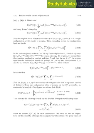
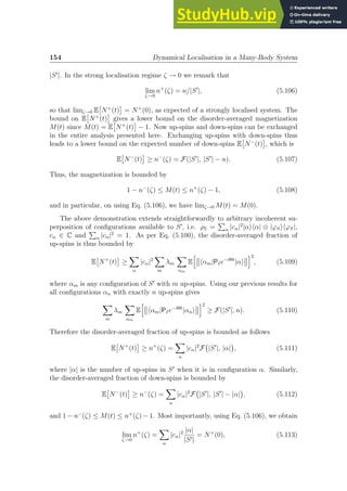
![5.8. Localisation of sublattice correlations 155
and similarly for E
N−
(t)
. These results thus show that for any ǫ ≥ 0, there exists
a localisation length ζ0 such that for all ζ ζ0, the magnetisation Mt of S′
is closer
to its initial value than ǫ, |M(t) − M(0)| ≤ ǫ.
5.8 Localisation of sublattice correlations
In this section we calculate the realisation average of the two time correlation func-
tion for any two sites i and j of S′
with I a bounded interval of energy
τi,j(t) = E
h
Tr[PIσi
z(t)PIσj
zρS]
i
, (5.114)
where ρS is the density matrix of the system. For the sake of clarity, from now on
we let |ωi denote |ωi ⊗ IS and similarly for |αi. First, we remark that
τi,j(t) = E
h
Tr
PIeiHt
(Ii
+ σi
z)e−iHt
PIσj
zρS
i
− Tr[σj
zρS], (5.115)
with Ii
the identity matrix on site i and Tr[σj
zρS] is the initial expectation of σj
z,
which is known. Now we consider the situation where ρS = |αihα| ⊗ |ϕSihϕS|. Then
E
h
Tr
PIeiHt
(Ii
+ σi
z)e−iHt
PIσj
zρS
i
= 2 (−1)δ↓j,α
X
ω: ↑i
E
h
Tr
hα|PIeiHt
|ωihω|e−iHt
PI|αi
i
,
= 2 (−1)δ↓j,α
X
ω: ↑i
E
h
khω|e−iHt
PI|αik2
F
i
, (5.116)
where the sum runs over configurations ω with an up-spin at site i and δ↓j, α = 1 if j
is down in α and 0 otherwise. Then, kAk2 ≤ kAkF together with Jensen’s inequality
gives
X
ω: ↑i
E
h
khω|e−iHt
PI|αik2
F
i
≥
X
ω: ↑i
E
h
khω|e−iHt
PI|αik
i2
. (5.117)
Now, in the localised phase, we know that for any two configurations α, ω and at any
time E
khω|PIe−iHt
|αik
≤ Ce−d(α, ω)/ζ0
for some positive ζ0. To progress, we assume
that there exists a localisation length ζ and time T such that for any t T, the
system saturates the localisation bounds on average, i.e. for any two configurations
α, ω and t T, we have E
khω|PIe−iHt
|αik
= Ce−d(α, ω)/ζ
. Then we have
X
ω: ↑i
E
h
khω|e−iHt
PI|αik2
F
i
≥
X
ω: ↑i
C2
e−2d(α,ω)/ζ
:= K(|S′
|, |α|), (5.118)](https://image.slidesharecdn.com/agraphtheoreticapproachtomatrixfunctionsandquantumdynamicsphdthesis-230805203656-4458b8ad/85/A-Graph-Theoretic-Approach-To-Matrix-Functions-And-Quantum-Dynamics-PhD-Thesis-165-320.jpg)
![156 Dynamical Localisation in a Many-Body System
where we have introduced K for later convenience. This quantity is explicitly given
by
K(|S′
|, |α|) = C2
δ↑i, α
|S′|−1
X
m=1
|S′|−1
X
d=0
N(|S′
| − 1, |α| − 1, m − 1, d)e−2d/ζ
+ C2
(1 − δ↑i, α)
|S′|−1
X
m=1
|S′|−1
X
d=1
N(|S′
| − 1, |α|, m − 1, d − 1)e−2d/ζ
, (5.119)
with δ↑i, α = 1 if α has an up-spin at site i and 0 otherwise and |α| is the number of
up-spins in S′
when it is in configurations α. We obtain this expression using the
results of the previous section. Indeed, recall that N(|S′
|, n, m, d) is the number of
configurations with m up-spins at distance d from a configuration with n up-spins
on the |S′
|-hypercube, see Eq. (5.104). Then the number of configurations with m
up-spins that have an up-spin at site i at distance d from a configuration with n
up-spins with an up-spin at site i is N(|S′
|−1, n−1, m−1, d). Similarly, the number
of configurations with m up-spins that have an up-spin at site i at distance d from a
configuration with n up-spins with a down-spin at site i is N(|S′
| − 1, n, m − 1, d −
1). We could not obtain an elegant form for the quantity K(|S′
|, |α|) although it
is straightforward to evaluate for a given value of |S′
| and fixed configuration α.
Finally, since K(|S′
|, |α|) ≥ 0 and for small ζ, K(|S′
|, |α|) ≤ 1, inserting Eq. (5.119)
into Eq. (5.115) gives
(
τi,j(t) ≤ 2K(|S′
|, |α|) − 1, if spin at site j is up in α,
τi,j(t) ≥ −2K(|S′
|, |α|) + 1, otherwise.
(5.120)
These bounds can be completed by another set of bounds obtained on repeating the
procedure presented above but starting with
τi,j(t) = Tr[σj
zρS] − E
h
Tr
PIeiHt
(Ii
− σi
z)e−iHt
PIσj
zρS
i
. (5.121)
We obtain
(
τi,j(t) ≥ −2Q(|S′
|, |α|) + 1, if spin at site j is up in α,
τi,j(t) ≤ 2Q(|S′
|, |α|) − 1, otherwise,
(5.122)
with
Q(|S′
|, |α|) = C2
(1 − δ↑i, α)
|S′|−1
X
m=1
|S′|−1
X
d=0
N(|S′
| − 1, |α| − 1, m − 1, d)e−2d/ζ
+ C2
δ↑i, α
|S′|−1
X
m=1
|S′|−1
X
d=1
N(|S′
| − 1, |α|, m − 1, d − 1)e−2d/ζ
. (5.123)](https://image.slidesharecdn.com/agraphtheoreticapproachtomatrixfunctionsandquantumdynamicsphdthesis-230805203656-4458b8ad/85/A-Graph-Theoretic-Approach-To-Matrix-Functions-And-Quantum-Dynamics-PhD-Thesis-166-320.jpg)
![5.9. Summary 157
Taken together Eqs. (5.120) and (5.122) guarantee that once our criterion for many-
body dynamical localisation holds for a sublattice comprising |S′
| sites, then the
correlation between any two spins of any such sublattice is localised in an interval
centered on its initial value.
5.9 Summary
We have established a natural criterion characterising dynamical localisation in in-
teracting many-body systems. Focusing on the XYZ Hamiltonian, which effectively
does not conserve the number of particles in the system, we have shown explicitly
that this criterion is fulfilled for a finite amount of disorder which scales at most
exponentially with the system size. Furthermore, once fulfilled, the criterion leads to
observable signatures of the localisation. In particular, we have bounded the mag-
netisation of any sublattice of a dynamically localised system and confirmed our
predictions with TEBD simulations. Similarly, we have shown that the correlations
between spins at the sites of the sublattice as well as the disorder-averaged magnetic
linear response function are constrained in the localised regime.
Our proof relies on the path-sums representation of the system generalised Green’s
functions. As we have seen in Chapters 2 and 3, this representation is independent
of the system Hamiltonian or system partition. For this reason, the proofs and
results presented here in the specific case of the XYZ-Hamiltonian hold in a much
more general setting. We hope that the path-sums representation, which allows the
systematic manipulation of system Green’s functions and generalised Green’s func-
tions, will contribute to the proof of localisation in infinite interacting many-body
systems.
The bound for σmin
B we obtain in Theorem 5.3.3 remains well above the critical
disorder observed in simulations, in particular in the XXZ regime where Jx = Jy.
To tighten the bound further will certainly require the explicit use of characteristic
features of the Hamiltonian. Similarly it may not be possible to prove dynamical
localisation of infinite interacting many-body systems without using specific prop-
erties that only some Hamiltonians exhibit. In particular, we believe that systems
whose spectrum exhibits persisting gaps in the thermodynamic limit are well suited
to proofs of dynamical localisation. Indeed in these situations, the moduli of the
entries of the evolution operators are expected to deterministically exhibit an expo-
nential decay as a function of distance on the configuration-space, i.e. even in the
absence of disorder [81, 82, 80]. While this effect is too weak to cause localisation by
itself, it might help control the divergences that appear when bounding the disorder
required for the onset dynamical localisation. Interestingly, recent results establish
deterministic exponential decay of functions of matrices over C∗
-algebra [84]. This
implies deterministic bounds for the norms of the generalised Green’s functions,
which are required to work with non-trivial system partitions S 6= ∅.](https://image.slidesharecdn.com/agraphtheoreticapproachtomatrixfunctionsandquantumdynamicsphdthesis-230805203656-4458b8ad/85/A-Graph-Theoretic-Approach-To-Matrix-Functions-And-Quantum-Dynamics-PhD-Thesis-167-320.jpg)

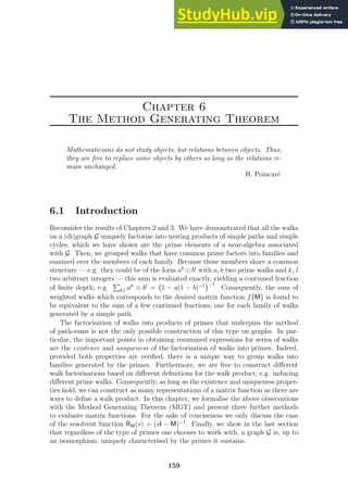
![160 The Method Generating Theorem
Method Walk product Primes Form of ΣWG; αω
Power-series Concatenation ◦ Edges Infinite sum
Primitive
series
Self-concatenation ˜
◦ Primitive orbits Infinite sum of fractions
Edge-sums Dual-nesting ¯
⊙ Edge-primes Finite continued fraction
Path-sums Nesting ⊙
Simple paths
cycles
Finite continued fraction
Language
equations
Incomplete nesting #
Simple paths
cycles
Finite system of equa-
tions
Table 6.1: Techniques for evaluating matrix functions stemming from the Method
Generating Theorem.
6.2 The method generating theorem
Theorem 6.2.1 (Method Generating Theorem). Let • be a walk product and W[.] a
weight function. Let SG be a subset of WG such that any walk of (SG, •) uniquely fac-
torises into products of prime walks and let F•(w) be the unique prime factorisation
of walk w. Then for any subset sG ⊆ SG,
X
w∈sG
w =
X
w∈sG
F•(w). (6.1a)
Furthermore, if SG = WG;αω and if W[
P
WG;αω
w] is finite, then
RM(s) = s−1
W[
X
WG; αω
s−ℓ(w)
F•(w)], (6.1b)
with ℓ(w) the length of walk w.
Proof. The theorem follows from a walk counting argument. By hypothesis the fac-
torisation a walks into products of prime walks always exists and is unique, there-
fore WG = {F•(w); w ∈ WG}. Then ΣG; αω =
P
w∈WG; αω
w =
P
w∈WG; αω
F•(w),
which is Eq. (6.1a). Supposing that W[ΣG; αω] exists, by virtue of Eq. (3.78b),
any partition of the resolvent function is given by a sum over weighted walks,
RM(s) = s−1
W[
P
WG; αω
s−ℓ(w)
w]. Thus, weighting Eq. (6.1a) gives Eq. (6.1b).
In spite of the apparent simplicity of the theorem, the MGT generates a rich
variety of methods, see Table 6.1. For example, consider applying the MGT with
the concatenation product: in this situation the prime elements of (WG, ◦) are the
graph edges (length 1 walks). Obviously F◦(w) always exist and is unique since it is
just w in edge notation and Eq. (6.1b) is the ordinary power-series expression of the
resolvent. The method of path-sums is another example of method that stems from](https://image.slidesharecdn.com/agraphtheoreticapproachtomatrixfunctionsandquantumdynamicsphdthesis-230805203656-4458b8ad/85/A-Graph-Theoretic-Approach-To-Matrix-Functions-And-Quantum-Dynamics-PhD-Thesis-170-320.jpg)
![6.3. Primitive series 161
the MGT, in this case with the walk product being the nesting product. As seen in
Chapters 2 and 3, Eq. (6.1b) now takes on the form of a continued fraction which
always exists on any finite graph. The nature (series, fractions, etc.) as well as the
convergence properties of the method so generated strongly depend on the extent to
which the series of factorised forms W[
P
WG; αω
F•(w)] lends itself to resummations.
In the next three sections, we present three further methods for evaluating series of
walks and matrix functions which stem from the MGT: primitive series, edge-sums
and language equations which generate matrix functions through series of fractions,
continued fractions and systems of equations, respectively.
6.3 Primitive series
A primitive orbit p′
(also called prime path and prime walk [174]) is a cycle which
is not a multiple of a shorter cycle, i.e. p′
is primitive if and only if there exists no
other cycle p such that p′
= pk
. We denote the set of all primitive orbits off vertex α
on G by PG; α. If G has at least two cycles with at least one vertex in common, then
PG; α is countably infinite. Primitive orbits are best known through their relations
with matrix determinants [175] and the Ihara zeta function [174]. Here we show
that primitive orbits are the prime elements induced by the self-concatenation walk
product which we define. Then, by the MGT, we recast the statics of any partition
of a resolvent as series of primitive orbits. We begin with the definition of a novel
walk-product: the self-concatenation.
6.3.1 The self-concatenation product
Definition 6.3.1 (Self-concatenation product). Let w = (αη2 · · · ηℓα) be a cycle of
length ℓ off α. Then the operation of self-concatenation is defined by
˜
◦ : WG × WG → WG, (6.2a)
(w, w′
) → w ˜
◦ w′
=
(
w ◦ w if w = w′
,
0 otherwise.
(6.2b)
The walk w ˜
◦ w of length 2ℓ consists of w concatenated with itself.
In the spirit of the path-algebra, the self-concatenation product induces an alge-
braic structure on cycle sets, the self-concatenation algebra:
Definition 6.3.2. The self-concatenation algebra KG˜
◦ = (
S
α∈V(G) WG;αα, +, ˜
◦ ) is
a noncommutative K-algebra whose support set is the set of cycles on G and with
the product of two cycles w, w′
given by the self-concatenation product w ˜
◦ w′
.
Proposition 6.3.1. The primitive orbits are the irreducible and prime elements of
KG˜
◦ . Furthermore, every cycle w on G factorises uniquely as
F˜
◦ (w) = pk
, (6.3)](https://image.slidesharecdn.com/agraphtheoreticapproachtomatrixfunctionsandquantumdynamicsphdthesis-230805203656-4458b8ad/85/A-Graph-Theoretic-Approach-To-Matrix-Functions-And-Quantum-Dynamics-PhD-Thesis-171-320.jpg)
![162 The Method Generating Theorem
where p is a primitive orbit and k ∈ N.
Proof. Irreducibility: let p ∈ PG and suppose p is reducible. Then, since w ˜
◦ w′
=
w2
δw,w′ , there exists p′
∈ PG and k ∈ N with p = (p′
)k
⇒ p /
∈ PG, a contradiction.
Existence: suppose that there exists a cycle w such that ∄ p ∈ PG with w = pk
,
k ∈ N. Then w is a primitive orbit and F˜
◦ (w) = w. Thus F˜
◦ (w) always exists.
Uniqueness: suppose that there exists a cycle w, two primitive orbits p1 and p2 and
two integers k1 and k2 such that w = pk1
1 = pk2
2 . Then, since w ˜
◦ w 6= 0, we have
p1 ˜
◦ p1 ˜
◦ · · · ˜
◦ p1 ˜
◦ p2 ˜
◦ · · · ˜
◦ p2 6= 0 and therefore p1 ˜
◦ p2 6= 0 ⇒ p1 = p2 and k1 = k2.
Thus F˜
◦ (w) is unique. Primality: let w and w′
be two cycles with w ˜
◦ w′
6= 0 and
let F˜
◦ (w ˜
◦ w′
) = (p′
)k
, p′
∈ PG. If p|w ˜
◦ w′
, then p|(p′
)k
and by the uniqueness of
the factorisation p = p′
. Since w ˜
◦ w′
6= 0, w = w′
and we have p|w. Thus p is
prime.
6.3.2 Primitive series for the resolvent
Having established the existence and uniqueness of the factorisation of cycles into
primitive orbits, we recast the resolvent into a primitive series using the MGT.
Theorem 6.3.1 (Primitive series for the resolvent). Let M ∈ CD×D
such that
ρ(M) s and {Mµν} be an arbitrary partition of M. Then the statics of the partition
of the resolvent RM(s) are given by the primitive series
RM(s)
α
=
1
s
h
1 +
X
p ∈ PG; α
W[p] sℓ
I − W[p]
−1
i
, (6.4)
with ℓ the length of the primitive orbit p.
Proof. On KG˜
◦ , the factorised form of any cycle is F˜
◦ (w) = pk
, Eq. (6.3). Then,
according to the MGT, when the series for the resolvent exists, i.e. ρ(M) s we
have
RM(s)
α
= s−1
W[(α) +
X
PG; α
X
k0
s−kℓ
pk
] = s−1
h
I +
X
PG; α
W[p] sℓ
I − W[p]
−1
, (6.5)
where (α) is the trivial walk off α. Convergence of the original power-series for
RM(s) is guaranteed when ρ(M) s and so is the convergence of the primitive
series. Additionally, if G has at least two cycles with at least one vertex in common,
then the primitive series above has a countably infinite number of terms. Therefore,
when ρ(M) ≥ s, convergence of the primitive series cannot be guaranteed.
6.3.3 Prime counting on graphs
A consequence of the existence of primitive series is the “graph-theory prime number
theorem”, which counts the primitive orbits of a graph and is usually proven via the
Ihara zeta-function [174].](https://image.slidesharecdn.com/agraphtheoreticapproachtomatrixfunctionsandquantumdynamicsphdthesis-230805203656-4458b8ad/85/A-Graph-Theoretic-Approach-To-Matrix-Functions-And-Quantum-Dynamics-PhD-Thesis-172-320.jpg)
![6.4. Edge-sums 163
Proposition 6.3.2 (Counting the primitive orbits of a graph). Let G be a digraph,
A is adjacency matrix and α a vertex of G. Then, the number πα(ℓ) of primitive
orbits of length ℓ 0 off α on G is
πα(ℓ) =
X
n|ℓ
µ ℓ/n
An
αα
, (6.6)
with µ(x) the Möbius function, defined as
µ(n) =
1, if n is a square-free positive integer with an even number of prime factors,
−1, if n is a square-free positive integer with an odd number of prime factors,
0, otherwise.
(6.7)
Remark 6.3.1. Usually, backtracks are omitted from the primitive orbits and one
counts unrooted primitive orbits rather than rooted ones, i.e. ℓ−1
πα(ℓ). The simple
proof provided here extends to this situation upon replacing A with Hashimoto’s
edge adjacency operator HHashimoto [174].
Proof. First, we express the walk generating function gG; αα(z) =
P
n zn
(An
)αα as a
primitive series. Since RM(s)
α
= s−1
gG; αα(s−1
), Theorem 6.3.1 yields
gG; αα(z) = 1 +
X
p∈PG; α
zℓ
1 − zℓ
= 1 +
X
ℓ
πα(ℓ)
zℓ
1 − zℓ
, (6.8)
where ℓ is the length of the primitive orbit. Equating powers of z in the above
expression with those of gG; αα(z) =
P
n zn
(An
)αα, we obtain (An
)αα =
P
ℓ|n πα(ℓ).
Then the Möbius inversion formula [176] gives the Proposition.
As noted by A. Terras in her book on zeta functions of graphs [174], the graph-
theory prime number theorem is much easier to obtain than its number theory
counterpart. This is because primitive orbits are not a good analogue to prime
numbers: by Proposition 6.3.1 every cycle w is either a primitive orbit or the multiple
of a unique primitive orbit. At the opposite, integers are generally divisible by more
than one prime. Then, counting primitive orbits is really equivalent to counting
integers that are not powers of other integers, n 6= pm
, p, m ∈ N∗
, a task much
easier than counting primes. A good graph theoretic analogue to prime numbers are
the simple cycles, since cycles are typically divisible by more than one simple cycle.
We observe that counting the simple cycles is indeed very hard: it is in fact a long
standing open problem [177], even on such simple graphs as Z2
.
6.4 Edge-sums
We have seen that the the prime walks appearing in the path-sums are walks forbid-
den from visiting any vertex more than once. Edge-sums is the edge-equivalent of](https://image.slidesharecdn.com/agraphtheoreticapproachtomatrixfunctionsandquantumdynamicsphdthesis-230805203656-4458b8ad/85/A-Graph-Theoretic-Approach-To-Matrix-Functions-And-Quantum-Dynamics-PhD-Thesis-173-320.jpg)
![164 The Method Generating Theorem
Directed
edge-dual
Figure 6.1: A digraph (left) and its directed edge-dual (right).
path-sums: it relies on prime walks that are forbidden from traversing any directed
edge more than once. We call these walks, edge-primes.
The validity of edge-sums follows directly from that of path-sums thanks to the
notion of directed edge-dual Ḡ of a graph G. The directed edge-dual is constructed
as follows: i) for each directed edge of G draw a vertex in Ḡ; and ii) place an edge
between two vertices of Ḡ if the directed edges of G corresponding to these two
vertices follow one another in G. An example of graph and its directed edge-dual is
represented in Figure 6.1. This construction implies that a walk on the directed edge-
dual w̄ ∈ WḠ is the directed edge-dual of a unique non-trivial walk on G. Thanks to
this relation, we define the dual-nesting product directly from the nesting product.
Definition 6.4.1 (Dual-nesting). Let (w1, w2) ∈ WG and (w̄1, w̄2) ∈ WḠ their
directed edge-duals. Then the dual-nesting of w1 with w2, denoted w1 ¯
⊙ w2, is the
walk whose directed edge-dual is w̄1 ⊙ w̄2.
The directed edge-duals of the primes induced by ¯
⊙ are simple paths and simple
cycles on Ḡ. Since a simple path/cycle does not visit any vertex of Ḡ more than
once, the primes induced by ¯
⊙ do not visit any directed edge more than once: there
are the edge-primes. Furthermore, since for any w̄ ∈ WḠ, the factorisation F⊙(w̄)
always exists and is unique, so is F¯
⊙(w) for any w ∈ WG. These observations
establish that edge-sums on G is path-sums on the directed edge-dual graph Ḡ.
Consequently, the edge-sum representation of the resolvent function is a continued
fraction of finite depth over the edge-primes, we omit the details. If G is a loopless
ordinary undirected connected graph, then the depth of this continued fraction is
equal to the length of the longest simple path on Ḡ. This is necessarily larger than
or equal to the length of the longest simple path on G, which reflects the fact that
there exists edge-primes which are not simple paths.
6.5 Language equations of matrix functions
Let Σ be a set of symbols, called an alphabet. Then a language L over Σ is any
subset of the Kleene star of Σ, denoted Σ∗
. The ensemble of rules satisfied by the
words of L is the grammar of L [32]. Words of L are generated by this grammar
through a set of equations, called the language equations [178, 179]. In this section](https://image.slidesharecdn.com/agraphtheoreticapproachtomatrixfunctionsandquantumdynamicsphdthesis-230805203656-4458b8ad/85/A-Graph-Theoretic-Approach-To-Matrix-Functions-And-Quantum-Dynamics-PhD-Thesis-174-320.jpg)
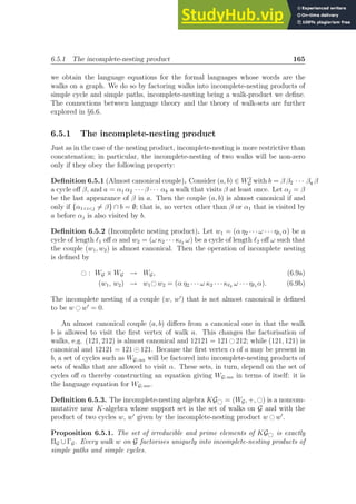
![166 The Method Generating Theorem
Proof. The proofs that KG# is a near K-algebra and Proposition 6.5.1 are entirely
similar to those given in §2.5.1 and §2.5.2, we omit the details. Note, the algorithm
that factorises walks into incomplete-nesting products of primes is nearly identical
to Algorithm 1. The only difference is that the new algorithm does not distinguish
cycles visiting their first vertex more than once from cycles that do not.
6.5.2 Language equations
Since all walks factorise uniquely into incomplete-nesting products of primes, the
MGT gives a novel factorised forms for walk-sets and sums of walks: the language
equations.
Theorem 6.5.1 (Language equations). The prime factorisation of WG into incomplete-
nesting products of sets of simple paths and simple cycles is achieved by the following
relations:
WG; ν0νp =
( ΠG; ν0νp # W∗
G{ν0,··· , νp−1}; νp
) # · · · # W∗
G{ν0}; ν1
# W∗
G; ν0
, (6.10a)
WG; µcµc =
( ΓG; µc # W∗
G{µ1,··· , µc−1}; µc
) # · · · # W∗
G{µ1}; µ2
# W∗
G; µ1
, (6.10b)
where (ν0 ν1 · · · νp−1 νp) ∈ ΠG; ν0νp and (µc µ1 · · · µc−1 µc) ∈ ΓG; µc .
Evaluating the incomplete-nesting products explicitly, we see that these equa-
tions involve the union ∪, the Kleene star ∗ and two-sided concatenations. The
weighted equivalent to Theorem 6.5.1 produces a set of equations fulfilled by the
desired matrix function. For the sake of conciseness, we present only the case of the
resolvent function.
Theorem 6.5.2 (Language equations for the resolvent). Let M ∈ CD×D
, {M}µν be
a partition of M and let G be the graph of this partition. Then the statics of the
partition of the resolvent RM(s) fulfill the equations
RM(s)
αω
=
X
ΠG; αω
RM; G{α,η2,··· ,ηℓ}(s)
ω
Mωηℓ
· · · RM(s)
η2
Mη2α RM(s)
α
, (6.11a)
RM(s)
α
=
X
ΓG; α
RM; G{η2,··· ,ηℓ}(s)
α
Mαηℓ
· · · Mη2η3 RM(s)
η2
Mη2α. (6.11b)
Remark 6.5.1 (Schützenberger methodology). The process of weighting the lan-
guage equations of Theorem 6.5.1 to obtain Theorem 6.5.2 is analogous to the
Schützenberger methodology [178]. This methodology was devised to count the
number of words in a language L defined through a formal grammar. It consists of
weighting the letters of an alphabet by a variable x and the words of L by xℓ
with ℓ
their length. Introducing these weights into the language equations for L and solving
them yields the generating function for the language. Clearly, this generating func-
tion is just the walk generating function on any graph G such that there exists two](https://image.slidesharecdn.com/agraphtheoreticapproachtomatrixfunctionsandquantumdynamicsphdthesis-230805203656-4458b8ad/85/A-Graph-Theoretic-Approach-To-Matrix-Functions-And-Quantum-Dynamics-PhD-Thesis-176-320.jpg)
![6.6. Unique characterisation of graphs 167
vertices α and ω and a bijective map Θ with Θ(WG;αω) = L and is consequently the
special case of Theorem 6.5.2 corresponding to x−1
RA(x−1
), with A the adjacency
matrix of G.
Example 6.5.1 (Language equations on P3). Consider the path-graph on three
vertices with a loop on each vertex, denoted P3. We label the vertices of the graph
1, 2 and 3. Using Theorem 6.5.1 we obtain the language equations for WP3; 11, WP3; 22
and WP3; 12 as follows:
WP3; 11 =
(1) ∪
(11) # W∗
P3; 11 ∪
(121) # W∗
P3; 22
# W∗
P3{2}; 11 , (6.12a)
WP3; 22 =
(2) ∪
(22) # W∗
P3; 22 ∪
(212) # W∗
P3; 11 ∪
(232) # W∗
P3; 33 , (6.12b)
WP3; 12 =
(12) # W∗
P3{1}; 22
# W∗
P3; 11}. (6.12c)
Remark how WP3; 11 and WP3; 22 are given in terms of their Kleene stars. This is also
true for WP3; 33 whose language equation is not shown here. The language equations
for the resolvent are obtained upon weighting Eqs. (6.12). Theorem 6.5.2 gives
RP3 (s)1 = 1 + w11RP3 (s)1 + RP3{2}(s)1 w12RP3 (s)2 w21, (6.13a)
RP3 (s)2 = 1 + w22RL2 (s)1 + RP3{1}(s)2 w21RP3 (s)1 w12 (6.13b)
+ RP3{3}(s)2 w23RP3 (s)3 w32,
where wνµ = W[(µν)] is the weight of edge (µν). Here again the statics of the
resolvent are given in terms of themselves and other resolvent statics.
6.6 Unique characterisation of graphs
Graphs are pervasive mathematical objects and an essential tool in the study of
large systems. Examples of applications abound where the analysis of complex
networks is paramount, ranging from understanding the structure of social relations
to evaluating the effects of medications on chains of protein reactions. Yet some basic
tasks such as distinguishing or quantifying the similarities between two networks
remain very difficult to perform and are the subject of active research in computer
science.
A remarkable result of automata theory asserts that a network is, up to an iso-
morphism, uniquely determined by the set of all walks on it [32]. Thus, in principle,
we can perfectly distinguish any two networks by comparing the walks they sustain.
This result is seldom used however, for there are infinitely many walks on typical
networks of interest. This difficulty is overcome by the fundamental result under-
lying the MGT and demonstrated in the thesis: there exists walk products such all
the walks on any graph factorize uniquely into products of prime walks. This obser-
vation reduces the difficulty of comparing the infinitely many walks of two networks
to comparing only their primes, of which there may be only a finite number, e.g.
the simple paths and simple cycles.](https://image.slidesharecdn.com/agraphtheoreticapproachtomatrixfunctionsandquantumdynamicsphdthesis-230805203656-4458b8ad/85/A-Graph-Theoretic-Approach-To-Matrix-Functions-And-Quantum-Dynamics-PhD-Thesis-177-320.jpg)
![168 The Method Generating Theorem
To establish this result rigorously, it is first necessary to describe graphs and
walks within the framework of language theory. Note, in this section we consider
only undirected, i.e. ordinary, graphs. For clarity, we defer all the proofs to §6.6.1.
Definition 6.6.1 (Alphabet on a graph). Let Σ be an alphabet and G a finite graph.
We say that Σ is an alphabet on G if and only if there exists a map Θ : E(G) → Σ
assigning labels to edges. We call Θ the labeling function.
Definition 6.6.2 (Automaton). An automaton A = (Q, Σ, δ, i, T) is a machine
with set of states Q, alphabet Σ, transition function δ, initial state i and final state
T. This automaton recognizes a language L if for all words w ∈ L, one can reach T
from i following transitions allowed by δ and labeled by letters of Σ.
Definition 6.6.3 (Minimal automaton). The minimal automaton A recognising a
language L is the automaton with the least number of states which recognises L.
Proposition 6.6.1 (Graphs as automata). Let G be a finite connected graph and α
and ω two vertices of G. Let Σ be an alphabet on G and Θ the corresponding labeling
function. Then the finite non-deterministic automaton
A(G)αω =
V(G), Σ, E(G), α, ω
, (6.14)
recognizes the language L ≡ Θ WG; αω
. Furthermore, if Θ is bijective, then A(G)αω
is the minimal automaton recognizing L.
Proposition 6.6.1 means that if we regard a walk-set WG; αω as a formal language
L, i.e. if we regard walks on G as words of L, then the graph G is the skeleton
(the structure) of a finite state machine, A(G)αω, which indicates whether a word
w belongs to L. Equivalently A(G)αω determines whether a walk w can be made
on G. Now a remarkable result from automata theory dictates that the minimal
automaton recognizing a language is unique up to an isomorphism [32]. This implies
an important result linking graphs and their walk-sets: the skeleton of the minimal
machine recognizing a language is uniquely determined by the walks on it.
Proposition 6.6.2 (Characterisation of graphs). Let G be a finite connected graph.
Then G is, up to an isomorphism, the unique graph with walk-sets {WG; αω}α,ω∈V(G).
In other terms, G is uniquely determined by its walk-sets.
Using this result to determine whether two graphs are isomorphic is hardly prac-
tical: it would entail comparing all the walks on the two graphs. But there are
typically infinitely many possible walks on graphs of interest. To resolve this diffi-
culty one needs to characterise uniquely the infinite set of all walks by finitely many
objects. This is precisely what we achieve using prime factorisations.
Theorem 6.6.1 (Prime characterisation of graphs). Let G be a finite connected
graph, • a walk product and PG the set of all primes induced by •. If the factorisation
F•(w) of a walk w ∈ WG into •-products of primes always exists and is unique, then
G is uniquely determined, up to an isomorphism, by the primes it sustains.](https://image.slidesharecdn.com/agraphtheoreticapproachtomatrixfunctionsandquantumdynamicsphdthesis-230805203656-4458b8ad/85/A-Graph-Theoretic-Approach-To-Matrix-Functions-And-Quantum-Dynamics-PhD-Thesis-178-320.jpg)
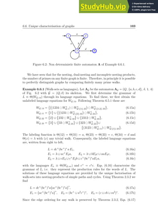
![170 The Method Generating Theorem
remains valid for non-commuting letters.
6.6.1 Proofs for the unique characterisation of graphs
◮ We first prove Proposition 6.6.1.
Proof. A(G)αω recognizes Θ WG; αω
: let Q ≡ V(G), δ ≡ E(G), and the initial state
i and final state T be respectively α and ω. Any walk w ∈ WG; αω, starts on i
and finishes on T. Furthermore, w only traverses edges e ∈ E(G), i.e. transitions
allowed by δ with label Θ(e) ∈ Σ, assuming Θ exists as in the proposition. The
walk w only visits vertices of V(G), i.e. states of the set Q of states available to the
automaton. Thus any word Θ(w) ∈ Θ WG; αω
is accepted by A(G)αω and Θ WG; αω
is recognized by A(G)αω.
A(G)αω is minimal for L ≡ Θ WG; αω
if Θ is bijective: an automaton A is the
minimal automaton recognizing a language if there exists no automaton B recogniz-
ing L with fewer states than A [32]. Suppose that there exists such an automaton B
with GB its skeleton and suppose first that GB is a subgraph of G. Then there exists
η ∈ V(G)V(GB). Since G is connected and undirected the set of walks WG;α→η→ω
from α to ω visiting η is non-empty and since Θ is bijective, there exists no walk
w′
∈ WG{η};αω such that Θ(w′
) = Θ(w). Thus the automaton B does not recognize
any word of Θ WG;α→η→ω
⊆ L and, consequently, does not recognize L, a contra-
diction. Now suppose that GB is not a subgraph of G. Since by hypothesis both
B(GB) and A(G)αω recognize L and since B(GB) is the minimal automaton for L,
it is isomorphic to a reduction of A(G)αω, i.e. GB is isomorphic to a subgraph of G.
As seen before, this leads to a contradiction.
◮ We now prove Proposition 6.6.2 and Theorem 6.6.1.
Proof. According to [32], the minimal automaton of a language is unique, up to an
isomorphism. Furthermore, by Proposition 6.6.1, A(G)αω is the minimal automaton
recognizing Θ WG; αω
for any bijective labeling function Θ. This means that A
is uniquely determined by Θ(WG; αω) and since Θ(.) is bijective, it is also uniquely
determined by WG; αω. Thus the skeleton G of A is uniquely determined by the
walks it sustains. This proves Proposition 6.6.2. Finally, in the situation where
∀ w ∈ WG, ∃!F•(w), Theorem 6.6.1 follows upon noting that any walk w ∈ WG has
a unique factorisation into products of primes, i.e. the set of all walks between any
two vertices of the graph is uniquely factorable into products of sets of primes.
6.7 Summary
In this chapter we have demonstrated the Method Generating Theorem, which as-
serts that if there exists a walk product operation • such that the prime factorisation
F•(w) of any walk w always exists and is unique, then there exists a universal rep-
resentation of formal walk series and matrix functions that only involves the primes
induced by the • product. Illustrating this result, we have presented three novel](https://image.slidesharecdn.com/agraphtheoreticapproachtomatrixfunctionsandquantumdynamicsphdthesis-230805203656-4458b8ad/85/A-Graph-Theoretic-Approach-To-Matrix-Functions-And-Quantum-Dynamics-PhD-Thesis-180-320.jpg)
![6.7. Summary 171
representations that also give rise to methods for evaluating matrix functions: the
primitive series, the edge-sums and the language equations. Finally, we have shown
that regardless of the walk product, a graph is uniquely characterised by the primes
it sustains.
The MGT offers remarkable freedom in the definition of walk products in spite of
the stringent constraints it imposes on the structure of walk-sets. It is already sur-
prising that walks on any digraph are uniquely factorable into prime elements, but
it is striking that this can be achieved in several ways, all simultaneously valid. Ad-
ditionally, the MGT shows that very little algebraic structure is required of (WG, •)
in order to design new representations of formal walk series and matrix functions.
Indeed, only the unique factorisation property is necessary. The weakness of this
requirement is truly remarkable, e.g. in the case of the nesting product, unique fac-
torisation holds at the individual walk level in spite of the product lacking a global
identity element and being neither commutative nor associative nor even distributive
with respect to addition. This stands in sharp contrast with the situation encoun-
tered in number theory where the uniqueness property is seemingly very fragile; a
fact that was fully recognized during the 19th century with the first examples of
number fields where uniqueness does not hold. This observation gave rise to the
notion of ideal, a concept of paramount importance in ring theory and abstract al-
gebra [39]. More recently, the study of unique factorisation and ideals was extended
to rings with zero divisors [180, 181], some noncommutative rings [182, 183, 40] and
nonassociative rings and algebras [184, 185]. So far, ideals of walks have not proven
necessary since the uniqueness is so much more robust for walks than for numbers.
Why this is so remains unclear. We propose that it is related to an intrinsic structure
that walks possess and numbers do not.](https://image.slidesharecdn.com/agraphtheoreticapproachtomatrixfunctionsandquantumdynamicsphdthesis-230805203656-4458b8ad/85/A-Graph-Theoretic-Approach-To-Matrix-Functions-And-Quantum-Dynamics-PhD-Thesis-181-320.jpg)

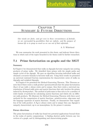
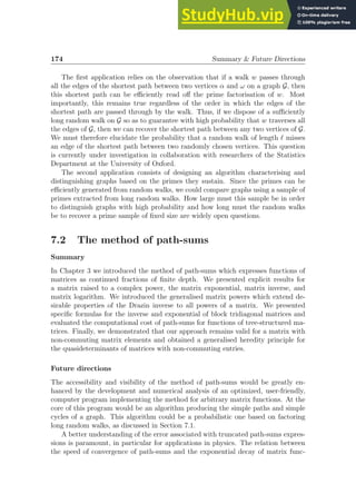
![7.3. Quantum dynamics and many-body Anderson localisation 175
tions must be clarified by future research. In this respect, the results of Chapter 5
represent a breakthrough. Indeed, the demonstration of Anderson localisation es-
tablishes that for “sufficiently random” matrices M: i) the weight of a fully dressed
simple path decays exponentially with its length, on average; and ii) this provokes
the exponential localisation of functions of M, on average. In their current form,
the arguments yielding these results do not extend to the deterministic case. They
point however to a remarkable competition taking place in infinite matrices between
the decay of simple path weights as a function of their length ℓ and the increase
of the number of simple paths of length ℓ as ℓ grows. When the decay dominates,
f(M) is exponentially localised around the sparsity pattern of M. In the opposite
situation, f(M) is non-negligible everywhere and everywhere difficult to calculate.
Physically, this would mean that the system approaches a phase transition, such as
from insulator to conductor, or more generally any quantum phase transition [186].
Finally, we mention the extension of the method of path-sums to the calculation
of functions of operators. In particular, we have developed a path-sum approach
for solving fractional differential equations which we could not report here due to
length concerns.
7.3 Quantum dynamics and many-body Ander-
son localisation
Summary
In the first part of Chapter 4, we derived the walk-sum lemma for the matrix-
exponential relying solely on physical arguments. We considered a quantum system
S to comprise two subsystems S and S′
and described the dynamics of S as a
superposition of walks undergone by S′
on a graph G. This graph is the discrete state
space of S′
: vertices represent configurations of S′
while edges represent physical
processes allowed by the Hamiltonian and which cause changes in the instantaneous
configuration of S′
. A walk of S on G thus represents a succession of configurations of
S′
, i.e. a walk is an history of S′
. The weight of this walk carries information about
the coupling between S and S′
or equivalently, the influence on S of the history of
S′
. The method of walk-sums is thus the discrete equivalent to Feynman’s path-
integrals: the dynamics of S results from the superposition of all histories available
to S′
. This gives a physical interpretation for path-sums in the context of quantum
dynamics: dressing vertices by cycles represents the dressing of S by virtual physical
processes undergone by S′
. Just as in quantum field theory, these processes give rise
to a non-zero self-energy, which in the path-sum description is simply a sum over
dressed simple cycles. In the second part of Chapter 4, we illustrated the method of
walk-sums by solving single particle continuous time quantum random walks. We
also investigated the dynamics of Rydberg-excited Mott insulators. In particular, we
demonstrated the existence of transient crystals formed by the Rydberg-excitations.
In Chapter 5, we demonstrated dynamical localisation of a strongly interacting](https://image.slidesharecdn.com/agraphtheoreticapproachtomatrixfunctionsandquantumdynamicsphdthesis-230805203656-4458b8ad/85/A-Graph-Theoretic-Approach-To-Matrix-Functions-And-Quantum-Dynamics-PhD-Thesis-185-320.jpg)
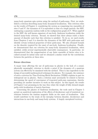

![Bibliography
[1] W. S. Bakr, J. I. Gillen, A. Peng, S. Fölling, and M. Greiner. A quantum
gas microscope for detecting single atoms in a Hubbard-regime optical lattice.
Nature 462, 74–77 (2009).
[2] J. F. Sherson, C. Weitenberg, M. Endres, M. Cheneau, I. Bloch, and S. Kuhr.
Single-atom-resolved fluorescence imaging of an atomic Mott insulator. Nature
467, 6872 (2010).
[3] W. S. Bakr, A. Peng, M. E. Tai, R. Ma, J. Simon, J. I. Gillen, S. Fölling,
L. Pollet, and M. Greiner. Probing the superfluid-to-Mott insulator transition
at the single-atom level. Science 329, 547–550 (2010).
[4] C. Weitenberg, M. Endres, J. F. Sherson, M. Cheneau, P. Schauß,
T. Fukuhara, I. Bloch, and S. Kuhr. Single-spin addressing in an atomic
Mott insulator. Nature 471, 319324 (2011).
[5] M. Lewenstein, A. Sanpera, V. Ahufinger, B. Damski, A. Sen De, and U. Sen.
Ultracold atomic gases in optical lattices: mimicking condensed matter physics
and beyond. Adv. Phys. 56, 243–379 (2007).
[6] R. P. Feynman. Simulating physics with computers. Int. J. Theor. Phys. 21,
467 (1982).
[7] S. Lloyd. Universal quantum simulators. Science 273, 1073 (1996).
[8] A. Steane. Multiple-particle interference and quantum error correction. Proc.
Roy. Soc. Lond. A 452, 2551 (1996).
[9] P. W. Shor. Algorithms for quantum computation: Discrete logarithms and
factoring. 35th Ann. IEEE Symp. Found. , 124 (1994).
[10] L. Grover. Quantum mechanics helps in searching for a needle in a haystack.
Phys. Rev. Lett. 79, 325 (1997).
[11] S. R. White. Density matrix formulation for quantum renormalization group.
Phys. Rev. Lett. 69, 28632866 (1992).
[12] J. I. Cirac and F. Verstraete. Renormalization and tensor product states in
spin chains and lattices. J. Phys. A - Math. Theor. 42, 504004 (2009).
[13] G. Vidal. Efficient classical simulation of slightly entangled quantum compu-
tations. Phys. Rev. Lett. 91, 147902 (2003).
178](https://image.slidesharecdn.com/agraphtheoreticapproachtomatrixfunctionsandquantumdynamicsphdthesis-230805203656-4458b8ad/85/A-Graph-Theoretic-Approach-To-Matrix-Functions-And-Quantum-Dynamics-PhD-Thesis-188-320.jpg)
![Bibliography 179
[14] F. Verstraete, V. Murg, and J. I. Cirac. Matrix product states, projected en-
tangled pair states, and variational renormalization group methods for quan-
tum spin systems. Adv. Theor. Phys. 57, 143–224 (2008).
[15] E. Jeckelman. Density-matrix renormalization group methods for momentum-
and frequency-resolved dynamical correlation functions. Prog. Theor. Phys.
Suppl. 176, 143–164 (2008).
[16] N. Shibata. Quantum hall systems studied by the density matrix renormal-
ization group method. Prog. Theor. Phys. Suppl. 176, 182–202 (2008).
[17] F. Verstraete and J. I. Cirac. Renormalization algorithms for quantum-many
body systems in two and higher dimensions. arXiv:cond-mat/0407066 [cond-
mat.str-el] (2004).
[18] Z.-C. Gu and X.-G. Wen. Tensor-entanglement-filtering renormalization ap-
proach and symmetry-protected topological order. Phys. Rev. B 80, 155131
(2009).
[19] P. Flajolet and R. Sedgewick. Analytic Combinatorics. Cambridge University
Press, Cambridge, 1st
edition, (2009).
[20] N. Biggs. Algebraic Graph Theory. Cambridge University Press, Cambridge,
2nd
edition, (1993).
[21] P. Flajolet. Combinatorial aspects of continued fractions. Discrete Math. 32,
125–161 (1980).
[22] C. D. Godsil. Algebraic Combinatorics. Chapman Hall, 1st
edition, (1993).
[23] D. J. Aldous and J. A. Fill. Reversible Markov Chains and Ran-
dom Walks on Graphs. (2003). Manuscript available electronically at
http://www.stat.berkeley.edu/users/aldous/RWG/book.html.
[24] J. R. Norris. Markov chains. Cambrigde University Press, Cambridge, 1st
edition, (1997).
[25] B. Bollobás. Modern Graph Theory. Springer, corrected edition, (1998).
[26] P. Blanchard and D. Volchenkov. Random Walks and Diffusions on Graphs
and Databases: An Introduction. Springer, 2011 edition, (2011).
[27] T. J. Sheskin. Markov Chains and Decision Processes for Engineers and Man-
agers. CRC Press, 1st
edition, (2010).
[28] H. C. Berg. Random walks in biology. Princeton University Press, Princeton,
revised edition, (1993).
[29] S. P. Borgatti, A. Mehra, D. J. Brass, and G. Labianca. Network analysis in
the social sciences. Science 323, 892–895 (2009).
[30] G. F. Lawler and V. Limic. Random walk : a modern introduction. Cambridge
University Press, Cambridge, 1st
edition, (2010).
[31] R. Burioni and D. Cassi. Random walks on graphs: ideas, techniques and
results. J. Phys. A - Math. Theor. 38, R45 – R78 (2005).](https://image.slidesharecdn.com/agraphtheoreticapproachtomatrixfunctionsandquantumdynamicsphdthesis-230805203656-4458b8ad/85/A-Graph-Theoretic-Approach-To-Matrix-Functions-And-Quantum-Dynamics-PhD-Thesis-189-320.jpg)
![180 Bibliography
[32] M. V. Lawson. Finite Automata. Chapman Hall/CRC, 1st
edition, (2004).
See in particular pp. 155-157.
[33] H. Dersken and J. Weyman. Quiver representations. Notices Amer. Math.
Soc. 52, 200–206 (2005).
[34] A. Savage. Finite-dimensional algebras and quivers. arXiv:math/0505082v1
[math.RA] (2005).
[35] J. Berstel and C. Reutenauer. Rational Series and Their Languages. Eatcs
Monographs on Theoretical Computer Science, electronic edition, (2008).
http://tagh.de/tom/wp-content/uploads/berstelreutenauer2008.pdf.
[36] I. M. Gel’fand, S. Gel’fand, V. Retakh, and R. Lee Wilson. Quasideterminants.
Adv. Math. 193, 56–141 (2005).
[37] H.-D. Ebbinghaus, J. Flum, and W. Thomas. Mathematical Logic. Springer,
New York, 2nd
edition, (1994).
[38] M. Auslander, I. Reiten, and S. O. Smalø. Representation Theory of Artin
Algebras. Cambridge University Press, Cambridge, 1st
edition, (1997).
[39] S. Lang. Algebra. Springer, 3rd
edition, (2002).
[40] T. Y. Lam. A first course in noncommutative rings. Springer, 2nd
edition,
(2001).
[41] G. S. Staples. A new adjacency matrix for finite graphs. Adv. Appl. Clifford
Alg. 18, 979–991 (2008).
[42] R. Schott and G. S. Staples. Operator calculus on graphs. Imperial College
Press, London, 1st
edition, (2012).
[43] G. H. Hardy and E. M. Wright. An introduction to the theory of numbers.
Oxford University Press, Oxford, 6th
edition, (2008).
[44] L. C. Eggan. Transition graphs and the star-height of regular events. Mich.
Math. J. 10, 385–397 (1963).
[45] H. Bethe. Statistical theory of superlattices. Proc. Roy. Soc. London Ser A
150, 552–575 (1935).
[46] R. J. Baxter. Exactly solved models in statistical mechanics. Academic Press,
1st
edition, (1982).
[47] C. Cai and Z. Y. Chen. Rouse dynamics of a dendrimer model in the ϑ
condition. Macromolecules 30, 5104–5117 (1997).
[48] Z. Y. Chen and C. Cai. Dynamics of starburst dendrimers. Macromolecules
32, 5423–5434 (1999).
[49] M. Droste and W. Kuich. Semirings and Formal Power Series in Handbook
of Weighted Automata, pp. 3 − 28. Springer, Berlin, Heidelberg, 1st
edition,
(2009).](https://image.slidesharecdn.com/agraphtheoreticapproachtomatrixfunctionsandquantumdynamicsphdthesis-230805203656-4458b8ad/85/A-Graph-Theoretic-Approach-To-Matrix-Functions-And-Quantum-Dynamics-PhD-Thesis-190-320.jpg)
![Bibliography 181
[50] J. Sakarovitch. Rational and Recognisable Power Series in Handbook of
Weighted Automata, pp. 105 − 174. Springer, Berlin, Heidelberg, 1st
edition,
(2009).
[51] N. J. Higham. Functions of Matrices: Theory and Computation. Society for
Industrial and Applied Mathematics, Philadelphia, 1st
edition, (2008).
[52] The On-Line Encyclopedia of Integer Sequences, 2013, http://oeis.org/.
[53] K. Ogata. Discrete-Time Control Systems. Prentice Hall, 2nd
edition, (1995).
[54] G. Meurant. A review on the inverse of symmetric tridiagonal and block
tridiagonal matrices. SIAM. J. Matrix Anal. Appl. 13, 707–728 (1992).
[55] R. K. Mallik. The inverse of a tridiagonal matrix. Linear Algebra Appl. 325,
109–139 (2001).
[56] E. Kılıç. Explicit formula for the inverse of a tridiagonal matrix by backward
continued fractions. Appl. Math. Comput. 197, 345357 (2008).
[57] G. Grosso and G. P. Parravicini. Solid State Physics. Elsevier, 2nd
edition,
(2014). See in particular pp. 27-34.
[58] H. Richter. Zum Logarithmus einer Matrix. Arch. Math. 2, 360–363 (1949).
[59] A. Wouk. Integral representation of the logarithm of matrices and operators.
J. Math. Anal. and Appl. 11, 131–138 (1965).
[60] S. L. Campbell and C. D. Meyer Jr. Generalized Inverses of Linear Trans-
formations. Society for Industrial and Applied Mathematics, Philadelphia,
(2009).
[61] N. J. Higham and L. Lin. On pth
roots of stochastic matrices. Linear Algebra
Appl. 435, 448–463 (2011).
[62] G. W. Cross and P. Lancaster. Square roots of complex matrices. Linear and
Multilinear Algebra 1, 289–293 (1974).
[63] A. Cayley. On certain results relating to quaternions. Philos. Mag. 26, 141–145
(1845).
[64] E. Study. Zur Theorie der linearen Gleichungen. Act. Math. 42, 1–61 (1920).
[65] A. Heyting. Die Theorie der linearen Gleichungen in einer Zahlenspezies mit
nichtkommutativer Multiplikation. Math. Ann. 98, 465–490 (1928).
[66] A. R. Richardson. Simultaneous linear equations over a division algebra. P.
Lond. Math. Soc. 55, 395–420 (1928).
[67] Ø. Ore. Linear equations in non-commutative fields. Ann. Math. 32, 463–477
(1931).
[68] I. M. Gel’fand and V. S. Retakh. Determinants of matrices over noncommu-
tative rings. Funct. Anal. Appl. 25, 91–102 (1991).
[69] I. M. Gel’fand and V. S. Retakh. A theory of noncommutative determinants
and characteristic functions of graphs. Funct. Anal. Appl. 26, 231–246 (1992).](https://image.slidesharecdn.com/agraphtheoreticapproachtomatrixfunctionsandquantumdynamicsphdthesis-230805203656-4458b8ad/85/A-Graph-Theoretic-Approach-To-Matrix-Functions-And-Quantum-Dynamics-PhD-Thesis-191-320.jpg)
![182 Bibliography
[70] I. M. Gel’fand and V. S. Retakh. Quasideterminants, i. Sel. Math. - New Ser.
3, 517–546 (1997).
[71] D. Krob and B. Leclerc. Minor identities for quasideterminants and quantum
determinants. Comm. Math. Phys. 169, 1–23 (1995).
[72] P. Etingof, I. Gel’fand, and V. Retakh. Factorization of differential operators,
quasideterminants, and nonabelian Toda field equations. Math. Res. Lett. 4,
413–425 (1997).
[73] P. Etingof, I. Gel’fand, and V. Retakh. Nonabelian integrable systems,
quasideterminants, and Marchenko lemma. Math. Res. Lett. 5, 1–12 (1998).
[74] P. Etingof and V. Retakh. Quantum determinants and quasideterminants.
Asian J. Math. 3, 345–351 (1998).
[75] C. R. Gilson and S. R. Macfarlane. Dromion solutions of noncommutative
Davey-Stewartson equations. J. Phys. A - Math. Theor. 42, 235202 (2009).
[76] M. Hassan. Darboux transformation of the generalized coupled dispersionless
integrable system. J. Phys. A - Math. Theor. 42, 065203 (2009).
[77] B. Haider and M. Hassan. Quasideterminant solutions of an integrable chiral
model in two dimensions. J. Phys. A - Math. Theor. 42, 355211 (2009).
[78] U. Saleem and M. Hassan. Quasideterminant solutions of the generalized
Heisenberg magnet model. J. Phys. A - Math. Theor. 43, 045204 (2010).
[79] A. Iserles. How large is the exponential of a banded matrix? New Zealand J.
Math. 29, 177–192 (2000).
[80] M. Benzi, P. Boito, and N. Razouk. Decay properties of spectral projectors
with applications to electronic structure. SIAM Review 55, 3–64 (2013).
[81] M. Benzi and G. H. Golub. Bounds for the entries of matrix functions with
application to preconditioning. BIT 39, 417–438 (1999).
[82] M. Benzi and N. Razouk. Decay bounds and O(n) algorithms for approx-
imating functions of sparse matrices. Electron. T. Numer. Ana. 28, 16–39
(2007).
[83] M. Cramer and J. Eisert. Correlations, spectral gap and entanglement in
harmonic quantum systems on generic lattices. New J. Phys. 8, 71 (2006).
[84] M. Benzi and P. Boito. Decay properties of functions of matrices over C∗
-
algebras. Linear Algebra Appl. , 25 (2013). DOI: 10.1016/j.laa.2013.11.027.
[85] C. Cohen-Tannoudji, J. Dupont-Roc, and G. Grynberg. Atom-Photon Inter-
actions. J. Wiley Sons, 1st
edition, (1998).
[86] G. Niestegge. An approach to quantum mechanics via conditional probabili-
ties. Found. Phys. 38, 241–256 (2008).
[87] Y. Aharonov, P. G. Bergman, and J. L. Lebowitz. Time symmetry in the
quantum process of measurement. Phys. Rev. 134, B1410B1416 (1964).](https://image.slidesharecdn.com/agraphtheoreticapproachtomatrixfunctionsandquantumdynamicsphdthesis-230805203656-4458b8ad/85/A-Graph-Theoretic-Approach-To-Matrix-Functions-And-Quantum-Dynamics-PhD-Thesis-192-320.jpg)
![Bibliography 183
[88] Y. Aharonov and L. Vaidman. Complete description of a quantum system at
a given time. J. Phys A - Math. Gen. 24, 2315 (1991).
[89] Y. Aharonov, L. Davidovich, and N. Zagury. Quantum random walks. Phys.
Rev. A 48, 1687 (1993).
[90] C. Moore and A. Russell. Quantum walks on the hypercube. Proc. 6th Int.
Workshop Rand. Approx. in Computer Science, LNCS 2483, Springer , 164
(2002).
[91] C. Moore and A. Russell. Quantum random walks hit exponentially faster.
Proc. 7th Int. Workshop Rand. Approx. in Computer Science, LNCS 2764,
Springer , 354 (2003).
[92] E. Farhi and S. Gutmann. Quantum computation and decision trees. Phys.
Rev. A 58, 915 (1998).
[93] A. M. Childs, R. Cleve, E. Deotto, E. Farhi, S. Gutmann, and D. A. Spiel-
man. Exponential algorithmic speedup by quantum walk. Proc. 35th ACM
Symposium on Theory of Computing , 59–68 (2003).
[94] N. Shenvi, J. Kempe, and K. Birgitta Whaley. Quantum random-walks search
algorithm. Phys. Rev. A 67, 052307 (2003).
[95] A. Childs, E. Farhi, and S. Gutmann. An example of the difference between
quantum and classical random walks. Quantum Information Processing 1, 35
(2002).
[96] J. Kempe. Quantum random walks - an introductory overview. Contemporary
Physics 44, 307 (2003).
[97] A. Ahmadi, R. Belk, C. Tamon, and C. Wendler. On mixing in continuous-
time quantum walks on some circulant graphs. Quantum Information and
Computation 3, 611 (2003).
[98] H. B. Perets, Y. Lahini, F. Pozzi, M. Sorel, R. Morandotti, and Y. Silber-
berg. Realization of quantum walks with negligible decoherence in waveguide
lattices. Phys. Rev. Lett. 100, 170506 (2008).
[99] A. Peruzzo, M. Lobino, J. Matthews, N. Matsuda, A. Politi, K. Poulios,
X. Zhou, Y. Lahini, N. Ismail, K. Worhoff, Y. Bromberg, Y. Silberberg,
M. Thompson, and J. O’Brien. Quantum walks of correlated photons. Science
329, 1193515 (2010).
[100] J. O. Owens, M. A. Broome, D. N. Biggerstaff, M. E. Goggin, A. Fedrizzi,
T. Linjordet, M. Ams, G. D. Marshall, J. Twamley, M. J. Withford, and A. G.
White. Two-photon quantum walks in an elliptical direct-write waveguide
array. New. J. Phys. 13, 075003 (2011).
[101] J. C. F. Matthews, K. Poulios, J. D. A. Meinecke, A. Politi, A. Peruzzo,
N. Ismail, K. Wörhoff, M. G. Thompson, and J. L. O’Brien. Simulating quan-
tum statistics with entangled photons: a continuous transition from bosons to
fermions. arXiv:1106.1166v1 [quant-ph] (2011).](https://image.slidesharecdn.com/agraphtheoreticapproachtomatrixfunctionsandquantumdynamicsphdthesis-230805203656-4458b8ad/85/A-Graph-Theoretic-Approach-To-Matrix-Functions-And-Quantum-Dynamics-PhD-Thesis-193-320.jpg)
![184 Bibliography
[102] L. Sansoni, F. Sciarrino, G. Vallone, P. Mataloni, A. Crespi, R. Ramponi, and
R. Osellame. Two-particle bosonic-fermionic quantum walk via integrated
photonics. Phys. Rev. Lett. 108, 010502 (2012).
[103] N. Goldman, A. Kubasiak, A. Bermudez, P. Gaspard, M. Lewenstein, and
M. A. Martin-Delgado. Non-Abelian optical lattices: Anomalous quantum
Hall effect and Dirac fermions. Phys. Rev. Lett. 103, 035301 (2009).
[104] A. Bermudez, L. Mazza, M. Rizzi, N. Goldman, M. Lewenstein, and M. A.
Martin-Delgado. Wilson fermions and axion electrodynamics in optical lat-
tices. Phys. Rev. Lett. 105, 190404 (2010).
[105] O. Boada, A. Celi, J. I. Latorre, and M. Lewenstein. Dirac equation for cold
atoms in artificial curved spacetimes. New J. Phys. 13, 035002 (2011).
[106] T. Kitagawa, M. S. Rudner, E. Berg, and E. Demler. Exploring topological
phases with quantum walks. Phys. Rev. A 82, 033429 (2010).
[107] L. Mazza, A. Bermudez, N. Goldman, M. Rizzi, M. A. Martin-Delgado, and
M. Lewenstein. An optical-lattice-based quantum simulator for relativistic
field theories and topological insulators. New. J. Phys. 14 (2012).
[108] R. C. Busby and W. Fair. Quadratic operator equations and periodic operator
continued fractions. J. Comput. Appl. Math. , 377–387 (1994).
[109] R. Vescovo. Inversion of block-circulant matrices and circular array approach.
IEEE T. Antenn. Propag. 45, 1565–1567 (1997).
[110] J. Anandan and Y. Aharonov. Geometry of quantum evolution. Phys. Rev.
Lett. 65, 1697–1700 (1990).
[111] V. Giovannetti, S. Lloyd, and L. Maccone. Quantum limits to dynamical
evolution. Phys. Rev. A 67, 052109 (2003).
[112] A. F. Andreev and I. M. Lifshitz. Quantum theory of defects in crystals.
Sov.Phys.-JETP 29, 1107–1113 (1969).
[113] G.V. Chester. Speculations on Bose-Einstein condensation and quantum crys-
tals. Phys. Rev. A 2, 256–258 (1970).
[114] A. J. Leggett. Can a solid be ”superfluid”? Phys. Rev. Lett 25, 1543–1546
(1970).
[115] E. Kim and M. H. W. Chan. Probable observation of a supersolid helium
phase. Nature 427, 225–227 (2004).
[116] V. W. Scarola, E. Demler, and S. Das Sarma. Searching for a supersolid in
cold-atom optical lattices. Phys. Rev. A 73, 051601(R) (2006).
[117] L. Pollet, J. D. Picon, H. P. Büchler, and M. Troyer. Supersolid phase with
cold polar molecules on a triangular lattice. Phys. Rev. Lett. 104, 125302
(2010).
[118] L. Bonnes and S. Wessel. Supersolid polar molecules beyond pairwise interac-
tions. Phys. Rev. B 83, 134511 (2011).](https://image.slidesharecdn.com/agraphtheoreticapproachtomatrixfunctionsandquantumdynamicsphdthesis-230805203656-4458b8ad/85/A-Graph-Theoretic-Approach-To-Matrix-Functions-And-Quantum-Dynamics-PhD-Thesis-194-320.jpg)
![Bibliography 185
[119] T. Keilmann, I. Cirac, and R. Roscilde. Dynamical creation of a supersolid in
asymmetric mixtures of bosons. Phys. Rev. Lett. 102, 255304 (2009).
[120] D. Jaksch, J. I. Cirac, P. Zoller, S. L. Rolston, R. Côté, and M. D. Lukin. Fast
quantum gates for neutral atoms. Phys. Rev. Lett. 85, 2208 (2000).
[121] I. Ryabtsev, D. Tretyakov, and I. Beterov. Applicability of Rydberg atoms to
quantum computers. J. Phys. B: At. Mol. Phys. 38, S421 (2005).
[122] M. Müller, I. Lesanovsky, H. Weimer, H. P. Büchler, and P. Zoller. Mesoscopic
Rydberg gate based on electromagnetically induced transparency. Phys. Rev.
Lett. 102, 170502 (2009).
[123] M. Saffman, T. G. Walker, and K. Molmer. Quantum information with Ryd-
berg atoms. arXiv:0909.4777v3 [quant-ph] (2010).
[124] M. Müller H. Weimer, I. Lesanovsky, P. Zoller, and H. P. Büchler. A Rydberg
quantum simulator. Nature Phys. 6, 382–388 (2010).
[125] H. Weimer H., R. Löw, T. Pfau, and H. Büchler. Quantum critical behavior
in strongly interacting Rydberg gases. Phys. Rev. Lett. 101, 250601 (2008).
[126] S. Ji, C. Ates, and I. Lesanovsky. Two-dimensional Rydberg gases and the
quantum hard squares model. Phys. Rev. Lett 107, 060406 (2011).
[127] I. Lesanovsky. Many-body spin interactions and the ground state of a dense
Rydberg lattice gas. Phys. Rev. Lett. 106, 025301 (2011).
[128] H. Weimer and H. Büchler. Two-stage melting in systems of strongly inter-
acting Rydberg atoms. Phys. Rev. Lett. 105, 230403 (2010).
[129] J. Schachenmayer, I. Lesanovsky, A. Micheli, and A. J. Daley. Dynamical
crystal creation with polar molecules or Rydberg atoms in optical lattices.
New J. Phys. 12, 103044 (2010).
[130] T. Pohl, E. Demler, and M. D. Lukin. Dynamical crystallization in the dipole
blockade of ultracold atoms. Phys. Rev. Lett. 104, 043002 (2010).
[131] M. Viteau, M. G. Bason, J. Radogostowicz, N. Malossi, D. Ciampini,
O. Morsch, and E. Arimondo. Rydberg excitations in Bose-Einstein conden-
sates in quasi-one-dimensional potentials and optical lattices. Phys. Rev. Lett.
107, 060402 (2011).
[132] T. F. Gallagher. Rydberg Atoms. Cambridge Monographs on Atomic, Molec-
ular and Chemical Physics. Cambridge University Press, (2005).
[133] T. Wilk, A. Gaëtan, C. Evellin, J. Wolters, Y. Miroshnychenko, P. Grang-
ier, and A. Browaeys. Entanglement of two individual neutral atoms using
Rydberg blockade. Phys. Rev. Lett. 104, 010502 (2010).
[134] J. Stanojevic and R. Côté. Many-body dynamics of Rydberg excitation using
the Ω-expansion. arXiv:0801.2396v1 (2008).](https://image.slidesharecdn.com/agraphtheoreticapproachtomatrixfunctionsandquantumdynamicsphdthesis-230805203656-4458b8ad/85/A-Graph-Theoretic-Approach-To-Matrix-Functions-And-Quantum-Dynamics-PhD-Thesis-195-320.jpg)
![186 Bibliography
[135] R. Heidemann, U. Raitzsch, V. Bendkowsky1, B. Butscher, R. Löw, L. Santos,
and T. Pfau. Evidence for coherent collective Rydberg excitation in the strong
blockade regime. Phys. Rev. Lett. 99, 163601 (2007).
[136] A. Gaëtan, Y. Miroshnychenko, T. Wilk, A. Chotia, M. Viteau, D. Comparat,
P. Pillet, A. Browaeys, and P. Grangier. Observation of collective excitation
of two individual atoms in the Rydberg blockade regime. Nat. Phys. 5, 115 –
118 (2009).
[137] G. G. Batrouni and R. T. Scalettar. Phase separation in supersolids. Phys.
Rev. Lett. 84, 1599–1602 (2000).
[138] P. Sengupta, L. P. Pryadko, F. Alet, M. Troyer, and G. Schmid. Supersolids
versus phase separation in two-dimensional lattice bosons. Phys. Rev. Lett.
94, 207202 (2005).
[139] P. W. Anderson. Absence of diffusion in certain random lattices. Phys. Rev.
109, 1492–1505 (1958).
[140] B. Kramer and A. MacKinnon. Localization: theory and experiment. Rep.
Prog. Phys. 56(12), 1469 (1993).
[141] D. Hundertmark. A short introduction to Anderson localization. Analysis
and Stochastics of Growth Processes and Interface Models, Oxford Scholarship
Online Monographs , 194–219 (2007).
[142] I. V. Gornyi, A. D. Mirlin, and D. G. Polyakov. Interacting electrons in
disordered wires: Anderson localization and low-T transport. Phys. Rev. Lett.
95, 206603 (2005).
[143] D. M. Basko, I. L. Aleiner, and B. L. Altshuler. Metal insulator transition in a
weakly interacting many-electron system with localized single-particle states.
Ann. Phys. 321(5), 1126 – 1205 (2006).
[144] V. Oganesyan and D. A. Huse. Localization of interacting fermions at high
temperature. Phys. Rev. B 75, 155111 (2007).
[145] M. Žnidarič, T. Prosen, and P. Prelovšek. Many-body localization in the
Heisenberg XXZ magnet in a random field. Phys. Rev. B 77, 064426 (2008).
[146] A. Karahalios, A. Metavitsiadis, X. Zotos, A. Gorczyca, and P. Prelovšek.
Finite-temperature transport in disordered Heisenberg chains. Phys. Rev. B
79, 024425 (2009).
[147] T. C. Berkelbach and D. R. Reichman. Conductivity of disordered quantum
lattice models at infinite temperature: Many-body localization. Phys. Rev. B
81, 224429 (2010).
[148] O. S. Barišić and P. Prelovšek. Conductivity in a disordered one-dimensional
system of interacting fermions. Phys. Rev. B 82, 161106 (2010).
[149] C. Monthus and T. Garel. Many-body localization transition in a lattice model
of interacting fermions: Statistics of renormalized hoppings in configuration
space. Phys. Rev. B 81, 134202 (2010).](https://image.slidesharecdn.com/agraphtheoreticapproachtomatrixfunctionsandquantumdynamicsphdthesis-230805203656-4458b8ad/85/A-Graph-Theoretic-Approach-To-Matrix-Functions-And-Quantum-Dynamics-PhD-Thesis-196-320.jpg)
![Bibliography 187
[150] I. L. Aleiner, B. L. Altshuler, and G. V. Shlyapnikov. A finite-temperature
phase transition for disordered weakly interacting bosons in one dimension.
Nature Physics 6(11), 900–904 (2010).
[151] A. Pal and D. A. Huse. Many-body localization phase transition. Phys. Rev.
B 82, 174411 (2010).
[152] E. Khatami, M. Rigol, A. Relaño, and A. N. Garcı́a-Garcı́a. Quantum
quenches in disordered systems: Approach to thermal equilibrium without
a typical relaxation time. Phys. Rev. E 85, 050102 (2012).
[153] C. Albrecht and S. Wimberger. Induced delocalization by correlations and
interaction in the one-dimensional Anderson model. Phys. Rev. B 85, 045107
(2012).
[154] M. Aizenman and S. Warzel. Localization bounds for multiparticle systems.
Commun. Math. Phys. 290, 903–934 (2009).
[155] B. Bauer and C. Nayak. Area laws in a many-body localized state and its
implications for topological order. arXiv:1306.5753 [cond-mat.dis-nn], (2013).
[156] B. L. Altshuler, Y. Gefen, A. Kamenev, and L. S. Levitov. Quasiparticle
lifetime in a finite system: A nonperturbative approach. Phys. Rev. Lett. 78,
2803–2806 (1997).
[157] E. Canovi, D. Rossini, R. Fazio, G. E. Santoro, and A. Silva. Quantum
quenches, thermalization, and many-body localization. Phys. Rev. B 83,
094431 (2011).
[158] G. Carleo, F. Becca, M. Schiró, and M. Fabrizio. Localization and glassy
dynamics of many-body quantum systems. Scientific reports 2 (2012).
[159] V. Chulaevsky and Y. Suhov. Multi-particle Anderson localisation: Induction
on the number of particles. Math. Phys. Anal. Geom. 12, 117–139 (2009).
[160] E. Abrahams, P. W. Anderson, D. C. Licciardello, and T. V. Ramakrishnan.
Scaling theory of localization: absence of quantum diffusion in two dimensions.
Phys. Rev. Lett. 42, 673 (1979).
[161] D. Hundertmark. On the time-dependent approach to Anderson localization.
Math. Nachr. 214, 25–38 (2000).
[162] S. Al-Assam, S. R. Clark, D. Jaksch, and TNT Development Team. TNT
Library Alpha Version, http://www.tensornetworktheory.org, (2012).
[163] D. Forster. Hydrodynamic fluctuations, broken symmetry, and correlation
functions. Addison-Wesley, 3rd
edition, (1990).
[164] M. Aizenman and S. Molchanov. Localization at large disorder and at extreme
energies: An elementary derivation. Commun. Math. Phys. 157, 245 (1993).
[165] M. Aizenman, J. H. Schenker, R. M. Friedrich, and D. Hundertmark. Finite-
volume fractional-moment criteria for Anderson localization. Commun. Math.
Phys. 224, 219–253 (2001).](https://image.slidesharecdn.com/agraphtheoreticapproachtomatrixfunctionsandquantumdynamicsphdthesis-230805203656-4458b8ad/85/A-Graph-Theoretic-Approach-To-Matrix-Functions-And-Quantum-Dynamics-PhD-Thesis-197-320.jpg)
![188 Bibliography
[166] H. Finner. A generalization of Hölder’s inequality and some probability in-
equalities. Ann. Probab. 20, 1893–1901 (1992).
[167] W. Kirsch. A Wegner estimate for multi-particle random hamiltonians.
arXiv:0704.2664v1 [math-ph], (2007).
[168] H. Bercovici B. Sz Nagy, C. Foias and L. Kérchy. Harmonic Analysis of
Operators on Hilbert Space. Springer, 2nd
edition, (2010).
[169] K.-J. Engel, R. Nagel, S. Brendle, and M. Campiti. One-Parameter Semi-
groups for Linear Evolution Equations. Springer, 1st
edition, (2000).
[170] M. Aizenman, A. Elgart, S. Naboko, J. H. Schenker, and G. Stolz. Mo-
ment analysis for localization in random Schrödinger operators. Invent. Math.
163(2), 343–413 (2006).
[171] R. Del Rio, S. Jitomirskaya, Y. Last, and B. Simon. Operators with singular
continuous spectrum, IV. Hausdorff dimensions, rank one perturbations, and
localization. J. Anal. Math. 69, 153–200 (1996).
[172] E. B. Saff and A. D. Snider. Fundamentals of Complex Analysis for Mathe-
matics, Science, and Engineering. Prentice Hall, 1st
edition, (1993).
[173] D. W. Wichern R. A. Johnson. Applied Multivariate Statistical Analysis. Pear-
son Higher Ed USA, 6th
edition, (2007).
[174] A. Terras. Zeta Functions of Graphs: A Stroll through the Garden. Cambridge
University Press, Cambridge, 1st
edition, (2011).
[175] R. Band, J. M. Harrison, and C. H. Joyner. Finite pseudo orbit expansions for
spectral quantities of quantum graphs. J. Phys. A - Math. Theor. 45, 325204
(2012).
[176] T. M. Apostol. Introduction to Analytic Number Theory. Springer, (2010).
[177] R. Bauerschmidt, H. Duminil-Copin, J. Goodman, and G. Slade. Lectures
on self-avoiding walks. In D. Ellwood, C. Newman, V. Sidoravicius, and W.
Werner, editors, Lecture notes, in Probability and Statistical Physics in Two
and More Dimensions, CMI/AMS Clay Mathematics Institute Proceedings,
2011.
[178] N. Chomsky and M. P. Schützenberger. The algebraic theory of context-free
languages. Comput. Prog. Form. Sys. 35, 118–161 (1963).
[179] E. L. Leiss. Language Equations. Springer, New York, reprint of the original
1st
ed. 1999 edition edition, (2012).
[180] S. Galovich. Unique factorization rings with zero divisors. Math. Mag. 51,
276–283 (1978).
[181] A. G. Agargün, D. D. Anderson, and S. Valdes-Leon. Unique factorization
rings with zero divisors. Commun. Algebra 27, 1967–1974 (1999).
[182] P. M. Cohn. Noncommutative unique factorization domains. Trans. Amer.
Math. Soc. 109, 313–331 (1963).](https://image.slidesharecdn.com/agraphtheoreticapproachtomatrixfunctionsandquantumdynamicsphdthesis-230805203656-4458b8ad/85/A-Graph-Theoretic-Approach-To-Matrix-Functions-And-Quantum-Dynamics-PhD-Thesis-198-320.jpg)
![Bibliography 189
[183] A. W. Chatters, M. P. Gilchrist, and D. Wilson. Unique factorization rings.
P. Edinburgh Math. Soc. 35, 255–269 (1992).
[184] B. Brown and N. H. McCoy. Prime ideals in nonassociative rings. Trans.
Amer. Math. Soc. 89, 245–255 (1958).
[185] P. J. Zwier. Prime ideals in a large class of non associative rings. Trans. Amer.
Math. Soc. 158, 257–271 (1971).
[186] S. Sachdev. Quantum Phase Transitions. Cambridge University Press, 2nd
edition, (2011).](https://image.slidesharecdn.com/agraphtheoreticapproachtomatrixfunctionsandquantumdynamicsphdthesis-230805203656-4458b8ad/85/A-Graph-Theoretic-Approach-To-Matrix-Functions-And-Quantum-Dynamics-PhD-Thesis-199-320.jpg)

This document is the doctoral thesis of Pierre-Louis Samuel Benoit Giscard submitted to the University of Oxford. The thesis develops a graph theoretic approach to matrix functions and quantum dynamics based on identifying an algebraic structure for sets of walks on graphs. It begins by establishing that walks on digraphs can be uniquely factored into products of prime elements, which are simple paths and cycles. This yields a continued fraction representation for the formal series of all walks on digraphs. The thesis then shows how common matrix functions can be expressed in terms of paths and cycles on the graph of the matrix's partition. Applications include simulating quantum random walks and Rydberg-excited systems. Overall, the thesis introduces a novel "