The document describes discrete Markov chains. A discrete Markov chain is a stochastic process that takes on countably many states, where the probability of moving to the next state depends only on the current state, not on the sequence of events that preceded it. This is known as the Markov property. The document defines discrete Markov chains mathematically and provides some basic properties, including the Markov property. It also gives examples of discrete Markov chains and how they can be specified by their transition probabilities between states.
![1. DISCRETE MARKOV CHAINS 1
1 Discrete Markov chains
Markov processes form an important class of random processes with many applications in areas
like physics, biology, computer science or finance. The characteristic property of a Markov
process is its lack of memory, that is, the decision where to go next may (and typically does)
depend on the current state of the process but not on how it got there. If the process can
take only countably many different values then it is referred to as a Markov chain.
1.1 Basic properties and examples
A stochastic process X = (Xt )t∈T is a random variable which takes values in some path space
S T := {x = (xt )t∈T : T → S}. Here, the space of possible outcomes S is some discrete (i.e.,
finite or countably infinite) state space and Xt is the state at time t (with values in S). In
this chapter, we will assume that time is discrete, i.e., we take the index set T to be the
non-negative integers N0 := {0, 1, 2, . . .}.
The distribution of X can be specified by describing the dynamics of the process, i.e., how
to start and how to proceed. By the multiplication rule, we have
P {(X0 , X1 , . . . , Xn ) = (x0 , x1 , . . . , xn )}
= P{X0 = x0 } P{X1 = x1 | X0 = x0 } P{X2 = x2 |X0 = x0 , X1 = x1 } · · ·
· · · P{Xn = xn | X0 = x0 , . . . , Xn−1 = xn−1 }
=: p0 (x0 ) p1 (x0 , x1 ) · · · pn (x0 , . . . , xn }. (1.1)
The left-hand side of equation (1.1) can be written as:
P{X ∈ Bx0 ,...,xn }, where Bx0 ,...,xn = {x0 } × {x1 } × · · · × {xn } × S {n+1,n+2,...} . (1.2)
Note that the functions pj , j ≥ 0 have to satisfy the following conditions.
1. pj (x0 , . . . , xj ) ≥ 0 for all j ≥ 0, x0 , . . . , xj ∈ S;
2. pj (x0 , . . . , xj ) = 1 for all j ≥ 0, x0 , . . . , xj−1 ∈ S.
xj ∈S
Remark. The measures in (1.1) uniquely extend to a probability measure on (S N0 , B),
where B is the σ-algebra generated by all sets of the form (1.2) (see Theorem 3.1 in [1]).
In general, the pj may depend on the entire collection x0 , . . . , xj . However, little can be said
about interesting properties of a stochastic process in this generality. This is quite different
for so-called Markovian stochastic dynamics, where the pj depend on xj−1 and xj only.
Definition 1.1 Let S be a countable space and P = (Pxy )x,y∈S a stochastic matrix (i.e.,
Pxy ≥ 0 and y∈S Pxy = 1, ∀ x ∈ S). A sequence of S-valued random variables (r.v.’s)
X0 , X1 , . . . is called a Markov chain (MC) with state space S and transition matrix P , if
P{Xn+1 = y | X0 = x0 , . . . , Xn−1 = xn−1 , Xn = x} = Pxy (1.3)
@ J. Geiger, Applied Stochastic Processes](https://image.slidesharecdn.com/scriptappl-111120141031-phpapp01/85/Applied-Stochastic-Processes-3-320.jpg)
![1. DISCRETE MARKOV CHAINS 19
We now turn to the question, under which circumstances we have the stronger convergence
P{Xn = y} → π(y) as n → ∞. We need some additional conditions as the following example
shows.
Consider symmetric SRW on Z2k for some k ∈ N. By symmetry, the uniform distribution
π(x) = (2k)−1 , x ∈ Z2k is the (unique) stationary distribution. However, Px {X2n+1 = x} = 0
for every n ∈ N0 . We will see, however, that this kind of periodicity is all that can go wrong.
Definition 1.23 A state x of a Markov chain with transition matrix P is called aperiodic if
n
gcd {n ≥ 1 : Pxx > 0} = 1.
A Markov chain is called aperiodic, if all states are aperiodic.
Lemma 1.24
n
i) x is aperiodic ⇐⇒ Pxx > 0 for all n sufficiently large.
ii) If (Xn )n≥0 is irreducible and some state is aperiodic, then the chain is aperiodic.
Proof.
i) A fundamental (and elementary) theorem from number theory states that, if A ⊂ N
is closed under addition and gcd A = 1, then N A is finite (for a proof see, e.g., the
n+k n k n
appendix of [2]). Clearly, Pxx ≥ Pxx Pxx . Hence, {n ≥ 1 : Pxx > 0} is such a set.
ii) Let z = x and suppose x is aperiodic. By the assumed irreducibility, states x and z
m
communicate, i.e., Pzx , Pxz > 0 for some , m ∈ N. Consequently,
+m+n n m
Pzz ≥ Pzx Pxx Pxz > 0
for all n sufficiently large. Part i) implies aperiodicity of z.
Theorem 1.25 (Convergence theorem) Let (Xn )n≥0 be an irreducible and aperiodic
Markov chain with stationary distribution π. Then
lim Px {Xn = y} = π(y) for all x, y ∈ S. (1.40)
n→∞
Remark. By the dominated convergence theorem, assertion (1.40) is equivalent to
lim dT V [Pµ {Xn ∈ · }, π] = 0
n→∞
for every initial distribution µ. (Recall that the total variation distance between probability
measures ρ1 and ρ2 on a discrete space S equals 1 x∈S |ρ1 (x) − ρ2 (x)|.)
2
Proof. The idea is to couple the chain (Xn )n≥0 with an independent chain (Yn )n≥0 which has
the same transition matrix P but initial distribution π, i.e., we will follow the path of (Xn )n≥0
until the two chains first meet, then follow the path of (Yn )n≥0 . The exact construction is as
follows.
@ J. Geiger, Applied Stochastic Processes](https://image.slidesharecdn.com/scriptappl-111120141031-phpapp01/85/Applied-Stochastic-Processes-21-320.jpg)
![28
2 Renewal processes
2.1 Limit theorems
+
Let Tj , j ≥ 1 be non-negative i.i.d. random variables with values in R0 and let T0 be a
R+ -valued random variable, independent of (Tj )j≥1 . Set S0 := 0 and
0
n
Sn+1 := T0 + Tj , n ≥ 0. (2.1)
j=1
The times Sn , n ≥ 1 are called renewal points. The number of renewals until time t is denoted
by
Nt := max{n ≥ 0 : Sn ≤ t}, t ≥ 0.
Note the relation
{Nt ≥ n} = {Sn ≤ t} for all n ∈ N and t ≥ 0.
Definition 2.1 The process (Yt )t≥0 with
Yt := SNt +1 − t, t ≥ 0,
is called a renewal process with lifetime distribution ν := L(T1 ) and delay T0 .
(Yt )t≥0 is the continuous-time analogue to the renewal chain studied in Chapter 1. Tradi-
tionally, the process (Nt )t≥0 is called renewal process. Note that in general the latter process
is not Markovian.
Proposition 2.2 (Law of large numbers) Suppose µ := E T1 ∈ (0, ∞], then
Nt 1
lim = a.s. (2.2)
t→∞ t µ
Proof. If P{T1 = ∞} = θ > 0 then Nt ↑ N∞ < ∞ a.s. as t → ∞, where
P{N∞ = k} = θ(1 − θ)k−1 , k ∈ N.
Hence,
Nt 1
=0=
lim a.s.
tt→∞ µ
Now assume P{T1 = ∞} = 0. By definition of Nt , we have SNt ≤ t < SNt +1 for all t ≥ 0.
Division by Nt gives
N t − 1 SNt t SNt +1
≤ < . (2.3)
Nt Nt − 1 Nt Nt
Now observe that
n
Sn+1 T0 j=1 Tj a.s.
i) = + → µ as n → ∞ (by the standard LLN);
n n n
a.s. a.s.
ii) Nt → ∞ (since Sn < ∞ for all n).
Asymptotics i) and ii) show that when passing to the limit t → ∞ in (2.3), both the lower
and upper bound converge to µ a.s.
@ J. Geiger, Applied Stochastic Processes](https://image.slidesharecdn.com/scriptappl-111120141031-phpapp01/85/Applied-Stochastic-Processes-30-320.jpg)
![2. RENEWAL PROCESSES 29
The function
∞ ∞
u(t) := ENt = P{Nt ≥ n} = P{Sn ≤ t}
n=1 n=1
is the so-called renewal function. The following theorem shows that we may interchange
expectation and limiting procedures in (2.2).
Theorem 2.3 (Elementary renewal theorem) Suppose that µ ∈ (0, ∞], then
u(t) 1
lim = .
t→∞ t µ
To prove Theorem 2.3 we need the following result which is interesting in its own.
Lemma 2.4 (Wald’s Identity) Let Z1 , Z2 , Z3 , . . . be i.i.d. random variables with E|Z1 | <
∞. Let τ be a stopping time for (Zn )n≥0 with E τ < ∞. Then
τ
E Zi = E τ EZ1 . (2.4)
i=1
τ
Relation (2.4) states that the mean of the random sum i=1 Zi is the same as if the Zi and
τ were independent.
Proof. Clearly,
τ ∞
Zi = Zi I{i ≤ τ }.
i=1 i=1
Note that
i−1
I{i ≤ τ } = 1 − I{τ ≤ i − 1} = 1 − I{τ = j}. (2.5)
j=0
Identity (2.5) and the fact that τ is a stopping time for (Zn ) show that the random variables
Zi and I{i ≤ τ } are independent. Thus (compare (1.17))
τ ∞
E Zi = E(Zi I{i ≤ τ })
i=1 i=1
∞
= EZi P{τ ≥ i}
i=1
∞
= EZ1 P{τ ≥ i} = EZ1 E τ.
i=1
1
Proof of Thm. 2.3. We may assume µ < ∞ (else u(t) ↑ u(∞) = θ < ∞). We first prove the
lower bound
u(t) 1
lim inf ≥ . (2.6)
t→∞ t µ
Since
n−1 n
{Nt = n} = {Sn ≤ t, Sn+1 > t} = Tj ≤ t < Tj
j=0 j=0
@ J. Geiger, Applied Stochastic Processes](https://image.slidesharecdn.com/scriptappl-111120141031-phpapp01/85/Applied-Stochastic-Processes-31-320.jpg)
![2. RENEWAL PROCESSES 31
2.2 Stationary renewal processes
This section deals with the question when the renewal process (Yt )t≥0 is a stationary process
(i.e., for what L(T0 )). By the Markov property, for (Yt )t≥0 to be stationary it is sufficient
that L(Yt ) does not depend on t. Now recall from Section 1.5 that if (Xn )n≥0 is an aperiodic,
irreducible and positive recurrent Markov chain then
Px {Xn = y} → π(y) as n → ∞ for all x, y ∈ S,
where π is the unique stationary distribution of (Xn )n≥0 . Hence, our opening question boils
down to finding the law of Yt = SNt +1 − t as t → ∞. Let
At := t − SNt
be the age of the item in use at time t. The first guess (?!) that the total lifetime TNt = At +Yt
of the item in use at t has asymptotic distribution ν = L(T1 ) is wrong. This is because of the
so-called size-biasing effect: It is more likely that t falls in a large renewal interval than that
it is covered by a small one.
To explain things in a simple setting we first have a look at stationary renewal chains (i.e.,
we take time to be discrete). Consider the augmented process (Yn , Zn )n≥0 , where Zn is the
total lifetime of the item in use at n. Observe that (Yn , Zn )n≥0 is a Markov chain on the state
space S = {(y, z) ∈ N2 : 0 ≤ y < z < ∞, qz > 0} with transition matrix
0
1, if y = y − 1, z = z,
P(y,z)(y ,z ) = qz , if y = 0, y = z − 1,
0, else.
Note that the chain (Yn , Zn )n≥0 is irreducible, since (y, z) → (0, z) → (z − 1, z ) → (y , z ).
Proposition 2.5 Suppose 0 < µ := ET1 = ∞ kqk < ∞. Then the stationary distribution
k=1
of the Markov chain (Yn , Zn )n≥0 is the distribution of the pair ( U T1 , T1 ), where T1 has the
size-biased distribution of T1 ,
y P{T1 = y}
P{T1 = y} = , y ∈ N0 ,
µ
and U is uniformly distributed on the interval [0, 1], independent of T1 .
2
Remark. Note that P{T1 ≥ 1} = 1 and that ET1 = ET1 /ET1 ≥ ET1 by Jensen’s inequality.
In fact, T1 is stochastically larger than T1 .
Proof. We first compute the weights of the distribution ( U T1 , T1 ) and then verify station-
arity. For 0 ≤ y < z < ∞ with qz > 0 we have
1
P{ U T1 = y | T1 = z} = P{ U z = y} = P{y ≤ U z < y + 1} = . (2.10)
z
@ J. Geiger, Applied Stochastic Processes](https://image.slidesharecdn.com/scriptappl-111120141031-phpapp01/85/Applied-Stochastic-Processes-33-320.jpg)
![2. RENEWAL PROCESSES 35
Theorem 2.11 (Blackwell’s renewal theorem) Suppose 0 < µ < ∞ and that L(T1 ) is
non-lattice. Then
h
u(t + h) − u(t) → as t → ∞
µ
for every h ≥ 0.
2.3 The homogeneous Poisson process on the half line
We now consider the case where the lifetimes Tj , j ≥ 1 have exponential distribution.
Definition 2.12 A non-negative random variable T is said to be exponentially distributed
with parameter λ > 0 (“Exp(λ)-distributed” for short), if
P{T ≥ t} = e−λt , t ≥ 0.
We list some elementary properties of the exponential distribution.
1. L(T ) has density f (t) = λe−λt , t ≥ 0.
2. T has mean E T = 1/λ and variance Var T = 1/λ2 .
3. The Laplace transform of T is
λ
ϕ(θ) := E exp(−θT ) = , θ ≥ 0.
λ+θ
4. The “lack of memory”:
P{T ≥ t + s | T ≥ t} = P{T ≥ s} for all s, t ≥ 0. (2.14)
Property (2.14) says that knowledge of the age gives no information on the residual lifetime.
This explains why in the case of exponential lifetimes the stationary density of T0 and the
lifetime distribution agree,
P{T1 > t}
g(t) = = λe−λt = f (t), t ≥ 0.
µ
This is commonly referred to as the bus stop paradox: If the interarrival times are exponen-
tially distributed then arriving at the bus stop at time t one has to wait as long as if arriving
immediately after a bus has left.
Definition 2.13 Let Tj , j ≥ 0 be independent Exp(λ)-distributed random variables. Then
the random set Φ := {Sn : n ≥ 1} is called a homogeneous Poisson process on R+ with
0
intensity λ.
The “homogeneous” refers to the process (Nt )t≥0 having stationary increments. The name
Poisson process is due to the following.
Proposition 2.14 Let N1 := | Φ ∩ [0, 1] | be the number of points of Φ in the unit interval.
Then
i) N1 is Poisson distributed with mean λ.
ii) Given N1 = n, the random variable (S1 , . . . , Sn ) is distributed like the order statistics
(U(1) , . . . , U(n) ) of n independent uniform random variables U1 , . . . , Un .
@ J. Geiger, Applied Stochastic Processes](https://image.slidesharecdn.com/scriptappl-111120141031-phpapp01/85/Applied-Stochastic-Processes-37-320.jpg)
![36
Recall that the order statistics is the Ui in increasing order. The respective assertions hold
for any interval [a, b].
Definition 2.15 A random variable X with values in the non-negative integers N0 is called
Poisson-distributed with parameter λ > 0, if
λk
P{X = k} = e−λ , k ∈ N0 .
k!
Sometimes it is convenient to have the case λ = ∞ included: The Poisson distribution with
parameter ∞ is the delta measure at ∞. We list some elementary properties of the Poisson
distribution.
1. X has mean EX = λ and variance Var X = λ.
2. The generating function of X is
EsX = e−λ(1−s) , 0 ≤ s ≤ 1.
3. The Poisson approximation of the binomial distribution B(n, pn ):
If npn → λ as n → ∞, then
n k λk
B(n, pn , k) = pn (1 − pn )n−k −→ e−λ as n → ∞.
k k!
Proof of Proposition 2.14. Let
B ⊂ {(s1 , s2 , . . . , sn ) : 0 ≤ s1 ≤ s2 ≤ . . . ≤ sn ≤ 1}
˜
be a measurable set. Write B for the corresponding inter arrival times,
˜
B := {(s1 , s2 − s1 , . . . , sn − sn−1 ) : (s1 , . . . , sn ) ∈ B}.
Then,
P{N1 = n, (S1 , . . . , Sn ) ∈ B}
= P((S1 , . . . , Sn ) ∈ B, Sn+1 > 1)
n
˜
= P (T0 , . . . , Tn−1 ) ∈ B, Tj > 1
j=0
= ˜
λe−λt0 λe−λt1 · · · λe−λtn dt0 · · · dtn
(t0 ,...,tn−1 )∈B,
t0 +···+tn >1
= λn λe−λsn+1 ds1 · · · dsn+1
(s1 ,...,sn )∈B, sn+1 >1
λn e−λ
= n! ds1 · · · dsn . (2.15)
n! B
@ J. Geiger, Applied Stochastic Processes](https://image.slidesharecdn.com/scriptappl-111120141031-phpapp01/85/Applied-Stochastic-Processes-38-320.jpg)
![2. RENEWAL PROCESSES 37
On the other hand,
P{(U(1) , . . . , U(n) ) ∈ B}
= P{(U(1) , . . . , U(n) ) ∈ B, Uρ(1) < Uρ(2) < · · · < Uρ(n) }
ρ permutation
= P{(Uρ(1) , . . . , Uρ(n) ) ∈ B}
ρ permutation
= n! P{(U1 , . . . , Un ) ∈ B}
= n! ds1 · · · dsn . (2.16)
B
Combining (2.15) and (2.16) establishes the claim of the proposition.
Observe that Proposition 2.14 suggests the following two-step construction of a homoge-
neous Poisson point process.
1. Choose a P oisson(λ)-distributed random number N , say.
2. Generate N independent uniform random variables on [0, 1].
Note that this construction has an obvious extension to more general state spaces (other than
the construction via lifetimes which uses the linear ordering of R). We will get back to this
construction in the next chapter.
2.4 Exercises
Exercise 2.1 (Stationary age processes) Consider a renewal chain (Yn )n≥0 with lifetime
distribution (qk )k≥1 and finite expected lifetime E T1 .
a) Compute the transition matrix of the time-reversed chain (compare Exercise 1.8 and
recall that π(y) = P{T1 > y}/ET1 , y ∈ N0 ).
b) Compute the so-called hazard function: the conditional probability that the lifetime T1
equals y given that it exceeds y.
Exercise 2.2 Let (Yt )t≥0 be a renewal process with renewal points Sn+1 = n Tj , n ≥ 0
j=0
and let X1 , X2 , . . . be a sequence of i.i.d. random variables with finite mean m := EX1 . The
renewal reward process is defined as
Nt
Rt := Xj , t ≥ 0.
j=1
a.s.
a) Let µ = ET1 be the expected lifetime. Show that Rt /t → m/µ.
b) Define At := t − SNt to the time at t since the last renewal (= age of the item in use).
Show that t 2
a.s. ET1
t−1 As ds −→ .
0 2µ
@ J. Geiger, Applied Stochastic Processes](https://image.slidesharecdn.com/scriptappl-111120141031-phpapp01/85/Applied-Stochastic-Processes-39-320.jpg)
![2. RENEWAL PROCESSES 39
e) Let X have (shifted) geometric distribution,
P{X = k} = p(1 − p)k , k ∈ N0 .
Show that
d d
X = 1 + X1 + X2 and U X = X,
where X1 and X2 are independent copies of X, and U is uniformly distributed on the
interval [0, 1], independent of X.
@ J. Geiger, Applied Stochastic Processes](https://image.slidesharecdn.com/scriptappl-111120141031-phpapp01/85/Applied-Stochastic-Processes-41-320.jpg)
![40
3 Poisson point processes
The Poisson point process is a fundamental model in the theory of stochastic processes. It is
used to model spatial phenomena (like the spread of colonies of bacteria on a culture medium
or the positions of visible stars in a patch of the sky) or a random series of events occurring
in time (like the emission of radioactive particles or the arrival times of phone calls).
Formally, a (Poisson) point process is a countable random subset of some state space S.
The distribution of Φ can be described by specifying the law of the number of points of Φ
falling into “test sets” Bi (where the Bi are from some σ-field B on S). To this end one needs
to ensure that there are enough sets in B. This can be done by the weak assumption that
the diagonal D = {(x, y) : x = y} is measurable in the product space (S × S, B ⊗ B), which
implies that singletons {x} are in B for every x ∈ S.
We will not address the measure theoretic niceties here (but be aware that there is some
demand !) and only list a few important properties (for a thorough account we refer to the
monographs [3, 6]).
• The set of countable subsets of a measurable set S is a Polish space when equipped with
the vague topology (identify Φ = {xi : i ∈ I} with the counting measure i∈I δxi ).
• The distribution of Φ is uniquely determined by the “finite-dimensional distributions”
of (N (B1 ), . . . , N (Bn )), where N (Bi ) := |Φ ∩ Bi | is the number of points that fall into
the set Bi .
3.1 Construction and basic properties
Definition 3.1 Let λ be a σ-finite (and non-atomic) measure on the measurable space (S, B).
A random countable subset Φ of S is called a (simple) Poisson point process on S with
intensity (or mean) measure λ, if
i) The random variables N (B1 ), . . . , N (Bn ) are independent for any finite collection of
disjoint measurable subsets B1 , . . . , Bn ∈ B.
ii) For every B ∈ B the random variable N (B) has Poisson distribution with mean λ(B).
Recall that a measure λ is called non-atomic if λ({x}) = 0 for all x ∈ S. This property is not
essential for the definition of a Poisson point process, but guarantees that Φ has no multiple
points. A measure λ is called σ-finite if there exist B1 ⊂ B2 ⊂ · · · ⊂ S such that i≥1 Bi = S
and λ(Bi ) < ∞ for all i, i.e., if S can be exhausted by sets of finite measure.
The inevitability of the Poisson distribution. We give a (somewhat heuristic) argu-
ment that the Poisson distribution is inevitable if one requires the maximal independence in
condition i) of Definition 3.1. Suppose that we independently throw points into the infinites-
imal volume elements dy with probability
P{N (dy) = 1} = EN (dy) = λ(dy).
@ J. Geiger, Applied Stochastic Processes](https://image.slidesharecdn.com/scriptappl-111120141031-phpapp01/85/Applied-Stochastic-Processes-42-320.jpg)
![50
c) Let Φ be a Poisson point process on R+ with intensity measure
α e−βz
λα,β (dz) = dz.
z
Show that
Y := x
x∈Φ
has distribution Gamma(α, β).
Exercise 3.4 PPP representation of the Gamma process. Let Φ be a Poisson point
process on R+ × R+ with intensity measure λ(ds dz) = ds λα,β (dz). Set
0
Yt := y, t ≥ 0.
(u,y)∈ Φ ∩ [0,t]
Show that:
a) Yt = limh↓0 Yt+h and Yt− := limh↓0 Yt−h exists a.s. for every t ≥ 0.
b) In every non-empty bounded time interval [t1 , t2 ] the process (Yt )t≥0 takes infinitely
many jumps, only finitely many of which exceed ε (> 0).
c) For every 0 ≤ t1 < t2 < · · · < tn+1 the increments Ytj+1 −Ytj , 1 ≤ j ≤ n are independent
random variables with distribution Gamma(α(tj+1 − tj ), β).
@ J. Geiger, Applied Stochastic Processes](https://image.slidesharecdn.com/scriptappl-111120141031-phpapp01/85/Applied-Stochastic-Processes-52-320.jpg)
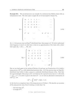
![4. MARKOV CHAINS IN CONTINUOUS TIME 51
4 Markov chains in continuous time
In this chapter time is continuous while the state space S is still discrete.
4.1 Definition and basic properties
Definition 4.1 Let P t , t ≥ 0 be a sequence of stochastic matrices on a discrete space S. A
stochastic process (Xt )t≥0 is called a (time-homogeneous) continuous-time Markov chain with
s
state space S and transition probabilities Pyz , if
s
Px {Xt+s = z | Xt1 = y1 , . . . , Xtn = yn , Xt = y} = Pyz (4.1)
for every n ∈ N0 , 0 ≤ t1 ≤ t2 ≤ . . . ≤ tn ≤ t, s ≥ 0 and x, y, y1 , . . . , yn , z ∈ S (provided that
the conditional probability is well defined). Here, Px is the law of (Xt )t≥0 when started at x.
Note that in the continuous-time setting we need a whole sequence of stochastic matrices to
describe the dynamics of the chain rather than a single transition matrix as in the discrete-
time case. The analogue of Lemma 1.3 are the so-called Chapman-Kolmogorov-equations:
The law of total probability and (4.1) imply that the P t satisfy
t+s
Pxy = Pxz Pzy = (P t P s )xy for all s, t ≥ 0 and x, y ∈ S.
t s
z∈S
In other words, the sequence P t , t ≥ 0 is a semigroup of stochastic matrices.
The distribution of the path (Xt )t≥0 is not uniquely determined by the finite-dimensional
distributions (4.1) as can be seen by the following example. Let
(1)
(Xt )t>0 ≡0
and
(2) 1, if t = U,
Xt =
0, else,
where U is uniformly distributed on the unit interval [0, 1], say. Both processes have transition
probabilities
t 1, if y = 0,
Pxy =
0, else.
In order to have uniqueness of L((Xt )t≥0 ) one has to require some smoothness of the paths
(e.g., that the paths are a.s. continuous or c`dl`g).
a a
4.2 Jump processes
Jump processes are an important class of Markov chains in continuous time. They can be
thought of as disrete-time Markov chains with randomized holding times.
Let T0 := inf{t > 0 : Xt = X0 } and assume Px {T0 > 0} = 1, i.e., the chain does not
instantaneously move away from its initial point (later on we will learn of processes where
this is not the case). The Markov property (4.1) then implies
Px {T0 ≥ t + s | T0 ≥ t} = Px {T0 ≥ t + s | Xu− = x for all 0 ≤ u ≤ t} = Px {T0 ≥ s}. (4.2)
@ J. Geiger, Applied Stochastic Processes](https://image.slidesharecdn.com/scriptappl-111120141031-phpapp01/85/Applied-Stochastic-Processes-53-320.jpg)
![4. MARKOV CHAINS IN CONTINUOUS TIME 53
Lemma 4.4 A (q, J)-jump process is regular if and only if
∞
1
Px =∞ = 1 for all x ∈ S.
qYn
n=0
Proof. We first consider the case where the embedded Markov chain (Yn )n≥0 is deterministic,
i.e., we assume that for each x ∈ S we have
x
Px { (Yn )n≥0 = (yn )n≥0 } = 1
x
for some (yn )n≥0 ∈ S N0 . In this case we need to show that
∞
1
Px {ζ = ∞} = 1 ⇐⇒ = ∞. (4.5)
q yn
x
n=0
For the necessity part of (4.5) observe that
∞ ∞ ∞
1
Ex ζ = Ex Tn = Ex Tn = .
q yn
x
n=0 n=0 n=0
Hence,
∞
1
< ∞ =⇒ Ex ζ < ∞ =⇒ Px {ζ < ∞} = 1.
q yn
x
n=0
For the other direction first observe that
Px {ζ = ∞} = 1 ⇐⇒ Ex exp(−ζ) = 0.
Clearly, we may assume qyn > 0 for all n. By the assumed independence of the Tn , we have
x
∞ ∞
Ex exp(−ζ) = Ex exp − Tn = Ex exp(−Tn )
n=0 n=0
∞
q yn
x 1 1
= = ≤ ∞ 1 .
1 + q yn
x ∞
1+ 1
n=0 qyx
n=0 n=0 q yn
x n
Hence,
∞
1
= ∞ =⇒ Ex exp(−ζ) = 0 =⇒ Px {ζ < ∞} = 1.
q yn
x
n=0
Now let (Xt )t≥0 have a general jump matrix J. By the law of total probability,
∞
Px {ζ = ∞} = Px Tn = ∞ = Ex g(Y0 , Y1 , . . .), (4.6)
n=0
where g : S N0 → [0, 1] is defined as
∞
g(y0 , y1 , . . .) := P Tn = ∞ Yn = yn , n ≥ 0 .
n=0
@ J. Geiger, Applied Stochastic Processes](https://image.slidesharecdn.com/scriptappl-111120141031-phpapp01/85/Applied-Stochastic-Processes-55-320.jpg)
![4. MARKOV CHAINS IN CONTINUOUS TIME 55
Is there a Markovian continuation of a non-regular (q, J)-jump process after its time of
explosion? In what follows we briefly discuss two possible extensions.
The minimal process. Let ∆ be some element not in S and set S ∆ := S ∪ {∆}. The
∆
minimal process (Xt )t≥0 following the dynamics (q, J) is constructed as above for all times
before ζ and is set equal to ∆ for times after the explosion (the absorbing external state ∆
is sometimes called cemetery). The minimal process is thus a continuous-time Markov chain
on S ∆ with transition probabilities
t
Pxy , x, y ∈ S;
∆t
Pxy = P{ζ ≤ t}, x ∈ S, y = ∆;
δxy , x = ∆.
Revival after explosion. Instead of letting the process being absorbed in the cemetery ∆
we can modify our (q, J)-jump process such that Px {Xt mod ∈ S} = 1 for all t ≥ 0: At time
of explosion let the process immediately jump back into S landing at z with probability ν(z)
where ν is some probability measure on S. At the next explosion we independently repeat
mod
this procedure (same ν !). The resulting process (Xt )t≥0 is a continuous-time Markov chain
on S whose distribution depends on ν.
4.4 Backward and forward equations
The backward and forward equations are two systems of differential equations for P t : R+ →0
t
[0, 1]. The idea behind is that, in general, computation of Pxy is difficult whereas computation
dP t
xy
of dt is easy. By the Markov property, those infinitesimal characteristics should contain
(almost) all information on the transition semi-group (P t )t≥0 .
Heuristics. We analyze P t near t = 0. Neglecting effects of multiple jumps (compare
Exercise 4.3) we have (recall our assumption Jxx ∈ {0, 1})
1 − Pxx = Px {T0 ≤ dt} = 1 − e−qx dt = qx dt
dt
(4.7)
and dt
Pxy = Px {T0 ≤ dt} Jxy = qx Jxy dt, x = y. (4.8)
The Q-matrix associated with q and J (or infinitesimal generator of the jump process (Xt )t≥0 )
is defined as
qx Jxy , if x = y,
Qxy :=
−qx , if x = y.
0
Note that q and J can be recovered from Q. Also, since Pxy = δxy , we can rewrite (4.7) and
(4.8) in matrix notation as
d t
P = Q. (4.9)
dt t=0
For the backward equations we decompose the evolution until time t + dt with respect to
Xdt , i.e., we write
P t+dt − P t = P dt P t − P t = (P dt − IdS )P t .
@ J. Geiger, Applied Stochastic Processes](https://image.slidesharecdn.com/scriptappl-111120141031-phpapp01/85/Applied-Stochastic-Processes-57-320.jpg)
![4. MARKOV CHAINS IN CONTINUOUS TIME 57
By (4.11), the first sum goes to zero as h ↓ 0 for each finite K, while the second sum can be
made arbitrarily small by choosing the set K large enough.
Hence, the product formula for differentiation yields
d t
P = −qx Pxy + e−qx t qx eqx t
t t
eJxz Pzy = t
Qxz Pzy . (4.13)
dt xy
z=x z∈S
For continuity of the derivative on the right-hand side of (4.13) recall (4.12).
Theorem 4.7 (Forward equations) Let (P t )t≥0 be the transition semi-group of a (q,J)-
jump process and assume
t
Pxy qy < ∞ (4.14)
y∈S
t
for all x, y ∈ S and t ≥ 0. Then Pxy is continuously differentiable with
d t t
P = Pxz Qzy . (4.15)
dt xy
z∈S
Remarks.
• The assertion of Theorem 4.7 holds without assumption (4.12) (see [10], pp.100–103 for
a proof).
• Condition (4.14) can be interpreted as the chain having finite expected speed at time t.
t
• For each fixed x ∈ S, (4.15) is a system of differential equations for vt := Px · .
Proof. For x = y we have
h
Pxy Px {T0 ≤ h} 1 − e−qx h
≤ = ≤ qx .
h h h
Also,
t+h t
Pxy − Pxy h
Pzy h
Pyy − 1
t t
= Pxz + Pxy .
h h h
z=y
Hence, by assumption (4.14) and the dominated convergence theorem,
t+h t
Pxy − Pxy h
Pzy h
Pyy − 1
t t t
lim = lim Pxz + Pxy lim = Pxz Qzy .
h↓0 h h↓0 h h↓0 h
z=y z∈S
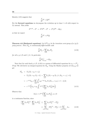
@ J. Geiger, Applied Stochastic Processes](https://image.slidesharecdn.com/scriptappl-111120141031-phpapp01/85/Applied-Stochastic-Processes-59-320.jpg)
![58
To stress the different role of the backward and forward equations consider a function
f : S → R and a measure µ on S. Note that
Ex f (Xt ) = Pxy f (y) =: (P t f )(x)
t
y∈S
is the expected payoff at t when started at x and that
Pµ {Xt = y} = µ(x)Pxy =: (µP t )(y)
t
x∈S
is the distribution of Xt when started with initial distribution µ. The function Pt f satisfies
the backward equations while the measure µt P satisfies the forward equations. Indeed,
d t d t t
(P f )(x) = P f (y) = f (y) Qxz Pzy
dt dt xy
y∈S y∈S z∈S
t
= Qxz Pzy f (y) = Qxz (P f )(z) =: (QP t f )(x).
t
z∈S y∈S z∈S
Similarly,
d
(µP t )(y) = (µP t Q)(y).
dt
The interchange of summation and differentiation has to be justified from case to case.
4.5 Stationary distributions
The notions of stationarity and ergodicity introduced in Chapter 1 have a natural extension
to the continuous-time setting. Also, the main results extend to continuous time with only
minor modifications.
Definition 4.8 A probability measure π on S is called a stationary distribution for (P t )t≥0 ,
if
πP t = π for all t ≥ 0.
Theorem 4.9 Suppose that the embedded chain (Yn )n≥0 is irreducible and positive recurrent
with stationary distribution ν. If (P t )t≥0 has a stationary distribution π, then
ν(x)
π(x) = c , x ∈ S,
qx
ν(y)
where c−1 = y∈S qy .
The result (see [2], pp. 358–359 for a proof) is not surprising in view of our interpretation of
π(x) as the asymptotic proportion of time that the chain spends in x. Note that ν(x) is the
asymptotic proportion of times at x while 1/qx is the expected time time spent at x per visit.
The following theorem is the continuous-time analogue of Theorem 1.25 (see Exercise 4.6
for a proof).
Theorem 4.10 (Convergence theorem) Let (Yn )n≥0 be an irreducible Markov chain and
suppose that (P t )t≥0 has stationary distribution π. Then,
t
lim Pxy = π(y) for all x, y ∈ S.
t→∞
@ J. Geiger, Applied Stochastic Processes](https://image.slidesharecdn.com/scriptappl-111120141031-phpapp01/85/Applied-Stochastic-Processes-60-320.jpg)
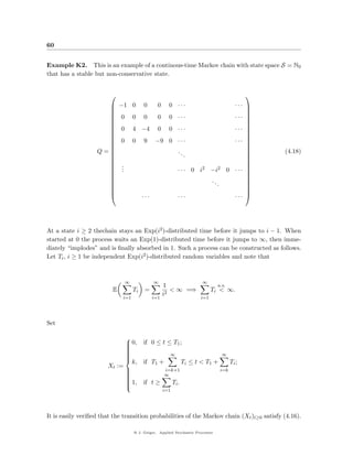
![4. MARKOV CHAINS IN CONTINUOUS TIME 59
4.6 Standard transition semi-groups
In Section 4.2 we obtained a semi-group of stochastic matrices starting from the description
of the dynamics of a continuous-time Markov chain in terms of the transition rates q and
the jump matrix J. Now we turn things around and start from the sequence of stochastic
matrices.
Definition 4.11 A sequence of stochastic matrices P t , t ≥ 0 is called a standard transition
semi-group on S, if
i) P 0 = IdS .
ii) P s+t = P s P t for all s, t ≥ 0.
h
iii) limh↓0 Pxx = 1 for all x ∈ S.
Properties i),–, iii) imply a great deal more than one might expect:
Theorem 4.12 Let (P t )t≥0 be a standard transition semi-group on S. Then
P h − IdS
lim =Q (4.16)
h↓0 h
exists with
−∞ ≤ Qxx ≤ 0 for all x ∈ S;
0 ≤ Qxy < ∞ for all x = y ∈ S;
y=x Qxy ≤ −Qxx for all x ∈ S. (4.17)
For a proof of Theorem 4.12, see [8], pp. 138–142.
Definition 4.13 A state x ∈ S is called
instantaneous, if Qxx = −∞,
stable , if Qxx > −∞.
A stable state x ∈ S is called
conservative, if Qxy = 0
y∈S
and non-conservative, else.
We will now discuss the probabilistic meaning of instantaneous and non-conservative states.
Note that the process has to jump away from an instantaneous state x immediately (since
Qxx = −∞). However, by the assumed continuity iii), the chain is at x for small times h
with probability close to 1. For a stable but non-conservative state x note that the process
should exit from S at the time it jumps away from x. However, since the P t are stochastic
matrices, it should immediately return.
The following two examples due to Kolmogorov illustrate these effects. They have become
known as K1 and K2. Starting from a Q-matrix which satisfies (4.17) (allowing Qxx = −∞ or
t
y Qxy < 0) we will construct a Markov chain (Xt )t≥0 . The associated semi-group (P )t≥0
will then be shown to satisfy (4.16).
@ J. Geiger, Applied Stochastic Processes](https://image.slidesharecdn.com/scriptappl-111120141031-phpapp01/85/Applied-Stochastic-Processes-61-320.jpg)


![Bibliography
[1] Billingsley, P. (1995) Probability and measure, 3rd ed., Wiley, Chichester.
[2] Bremaud, P. (1999) Markov chains. Gibbs fields, Monte Carlo simulation, and queues.
´
Springer, New York.
[3] Daley, D.J. and Vere-Jones, D. (1988). An introduction to the theory of point
processes. Springer, New York.
[4] Durrett, R. (1999). Essentials of stochastic processes. Springer, New York.
[5] Haggstrom, O. (2002). Finite Markov chains and algorithmic applications, Cambridge
¨ ¨
University Press, Cambridge.
[6] Kallenberg, O. Foundations of modern probability. 2nd ed. Springer, New York.
[7] Karlin, S. and Taylor, H. M. (1975). A first course in stochastic processes, 2nd ed.
Academic Press, New York.
[8] Karlin, S. and Taylor, H. M. (1981). A second course in stochastic processes. Aca-
demic Press, New York.
[9] Kingman, J.F.C. (1993). Poisson processes. Clarendon Press, Oxford.
[10] Norris, J. R.(1997). Markov chains. Cambridge University Press, Cambridge.
69](https://image.slidesharecdn.com/scriptappl-111120141031-phpapp01/85/Applied-Stochastic-Processes-71-320.jpg)


