This document presents a general method for estimating unknown coefficients in linear structural equation systems, accommodating both errors in equations and errors in variables. The method allows for the computation of residual variance-covariance matrices and measurement error variances, and it includes an illustrative application to economic and psychological data. Additionally, it discusses two special cases involving either errors in equations or errors in variables and outlines the numerical methods and assumptions used for estimation.

1. A GENERAL METHOD FOR ESTIMATING A LINEAR STRUCTURAL
R
~
(
A
R
~ ~
T
I
N
EQUATION SYSTEM
II
Karl G. Joreskog
RB-70-54
This Bulletin is a draft for interoffice circulation.
Corrections and suggestions for revision are solicited.
The Bulletin should not be cited as a reference without
the specific permission of the author. It is automati-
cally superseded upon formal publication of the material.
Educational Testing Service
Princeton, New Jersey
September 1970

2. A General Method for Estimating a Linear Structural
Equation System
Karl G. J8reskog
Educational Testing Service
Abstract
A general method for estimating the unknown coefficients in a set
of linear structural equations is described. In its most general form the
method allows for both errors in equations (residuals, disturbances) and
errors in variables (errors of measurement, observational errors) and yields
estimates of the residual variance-covariance matrix and the measurement error
variances as well as estimates of the unknown coefficients in the structural
equations, provided all these parameters are identified. Two special
cases of this general method are discussed separately. One is when there
are errors in equations but no errors in variables. The other is when there
are errors in variables but no errors in equations. The methods are applied
and illustrated using artificial, economic and psychological data.

3. A General Method for Estimating a Linear Structural
Equation System*
1. Introduction
We shall describe a general method for estimating the unknown coe~ficients
in a set of linear structural equations. In its most general form the method
will allow for both errors in equations (residuals, disturbances) and errors
in variables (errors of measurement, observational errors) and will yield
estimates of the residual variance-covariance matrix and the measurement error
variances as well as estimates of the unknown coefficients in the structural
equations, provided all .these parameters are identified. After giving
the results for this general case, two special cases will be considered.
The first is the case when there are errors in equations but no errors in
variables. This case has been studied extensively by econometricians (see
e.g., Goldberger, 1964, Chapter 7). The second case is when there are
errors in variables but no errors in equations. Models of this kind have
been studied under the name of path analysis by biometricians (see e.g.,
Turner & Stevens, 1959») sociologists (see e.g., Blalock, 1964) and psycholo-
gists (Werts & Linn, 1970).
It is assumed that the observed variables have a multinormal distribu-
tion and the unknmYn parameters ar~ estimated by the maximum likelihood method.
The estimates are computed numerically using a modi~ication of the Fletcher-
Powell minimization algorithm (Fletcher & Powell, 1963; Gruvaeus &JBreskog,
1970). Standard errors of the estimated parameters may be obtained by
computing the inverse of the information matrix. A computer program,
*This research has been supported in part by grant NSF-GB-12959 from the
National Science Foundation. The author wishes to thank Professor Arthur
Goldberger for his . comments on an earlier draft of the paper and Marielle
van Thillo, who wrote the computer programs, checked the mathematical
derivations and gave other valuable assistance throughout the work.

4. -2-
LISREL, in FORTRAN IV, that performs all the necessary computations has been
written and tested out on the IBM 360/65; a write-up of this is under
preparation (J8reskog & van Thillo, 1970).
In the first special case referred to above, where there are no errors
of measurement in the observed variables the general method to be presented
is equivalent to the full information maximum likelihood (FIML) method of
Koopmans, Rubin and Leipnik (1950) also called full information least
generalized residual variance (FILGRV) method (Goldberger, 1964, Chapter 7),
provided that no constraints are imposed on the residual variance-covariance
matrix and the variance-covariance matrix of the independent variables.
However, with the general method described here, it is possible to assign
fixed values to some elements of these matrices and also to have equality
constraints among the remaining elements.
2. The General Model
Consider random vectors ~t ~ (~1'~2' •• ·'~) and S' ~ (Sl'S2' ••• 'Sn)
of true dependent and independent variables, respectively, and the following
system of linear structural relations
(1)
where B(m x m) and ~(m x n) are coefficient matrices and ~I ~ (~l' ~, ••• ,
Sm) is a random vector of residuals (errors in equations, random disturbance
terms). Without loss of generality it may be assumed that e(~) = e(~)~ Q
and e(~) ~ o. It is furthermore assumed that S is uncorrelated with
s and that ~ is nonsingular.

5. -3-
The vectors ~ and e are not observed but instead vectors yl =
(Yl'Y2'·"'Ym) and Xl = (xl,x2, ... ,x
n)
are observed, such that
Y (2)
x=v+~+5
where I-l = ,e(y) v = e(~) and E and 5 are vectors of errors of measure-
ment in y and ~, respectively. It is convenient to refer to y and x
as the observed variables and ~ and s as the true variables. The errors
of measurement are assumed to be uncorrelated with the true variates and
among themselves.
Let p(n x n) and
and s} respectively,
be the variance-covariance matrices of
8
2
the diagonal matrices of error
_5
variances for y and ~, respectively. Then it follows, from the above
assumptions, that the variance-covariance matrix E[(m + n) x (m + n)] of
z = (y"::5 r )' is
(4)
~-l~~1~1-l
E =f -
~::.~.-l
The elements of E are functions of the elements of B} r, ¢, ~,
and 8 .
~E
In applications some of these elements are fixed and equal
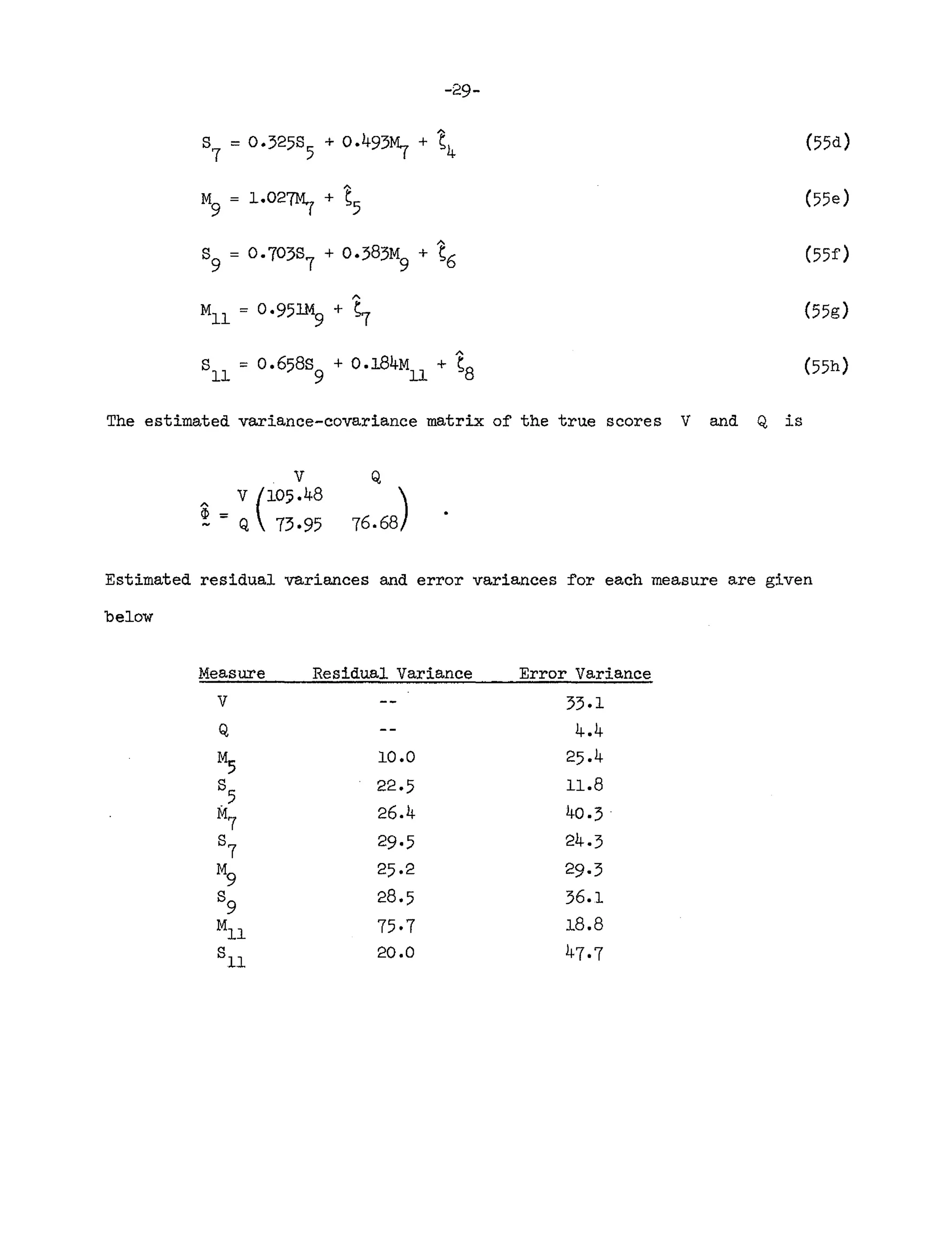
to assigned values. In particular this is so for elements in B
- and I' '
but we shall allow for fixed values even in 'the other matrices. For the
remaining nonfixed elements of the six parameter matrices one or more subsets
may have identical but unknown values. Thus parameters in B, E', p,
0/ , and s
~E
are of three kinds: (i) fixed parameters that have been

6. -4-
assigned given values, (ii) constrained parameters that are unknown but equal
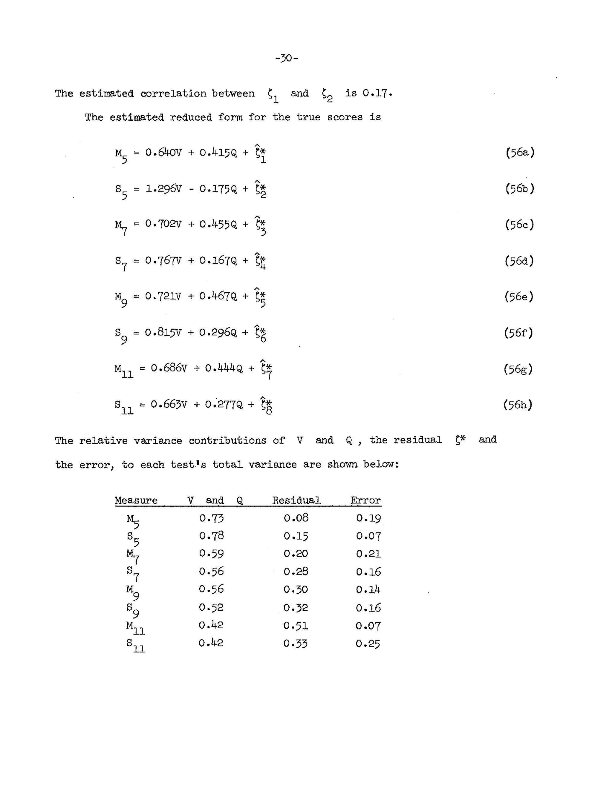
to one or more other parameters and (iii) free parameters that are unknown and
not constrained to be equal to any other parameter.
Before an attempt is made to estimate a model of this kind, the identi-
fication problem must be examined. The identification problem depends on
the specification of fixed, constrained and free parameters. Under a given
specification, a given structure ~' r} ~, t, ~5} (3 generates
-€
one and only one ~ but there may be several structures generating the
same ~. If two or more structures generate the same ~, the structures
are said to be equivalent. If a parameter has the same value in all equiva-
lent structure~ the parameter is said to be identified. If all parameters
of the model are identified, the whole model is said to be identified. When
a model is identified one can usually find consistent estimates of all its
parameters. Some rules for investigating the identification problem when
there are no errors in variables are given by Goldberger (1964, pp. 306-318).
3. Estimation of the General Model
Let ~1'~2' ···}~N be N observations of z = (~t}~t)J • Since no
constraints are imposed on the mean vector (~t,yr)r the maximum likelihood
ti th · · t t z = (y-', x- t ) t
es mate of 1S 1S he usual sample mean vec or •
1 N
§ = - ~ (z~ - ~)(~a - ~),
N a=l "'U
be the usual sample variance-covariance matrix, partitioned as
Let
~[(m + n) x (m + n)]
=[~yy(m x m)
S (n x m)
~xy
S (m x
~yx
S (n x
-xx
n)j
n)
(6)

7. -5-
The logarithm of the likelihood function, omitting a function of the
observations, is given by
This is regarded as a function of the independent distinct parameters
in B, r , ~, IF, e and e and is to be maximized with respect
-0 -e
to these, taking into account that some elements may be fixed and some
may be constrained to be equal to some others. Maximizing log L is equiva-
lent to minimizing
(8)
Such a minimization problem may be formalized as follows.
Let At ~ (~,~, ••• ,Ap) be a vector of all the elements of ~, r
~, IF, e and 8 arranged in a prescribed order. Then F may be
.- _0 -E
regarded as a function
continuous derivatives
F(~)
of/OAs
of ~,A2""'"
and o~/Oo
which is continuous and has
of first and second order,
except where ~ is singular. The totality of these derivatives is repre-
sented by a gradient vector OF/O~ and a symmetric matrix o2F/Of}J~t • Now
let some p - q of the A's be fixed and denote the remaining A's by ~l'
~2""'~q' q ~ p. The function F is now considered as a function G(~)
of ~1'~2""'~q' Derivatives OG/O~ and 02G/d~d~' are obtained from
OF/d?:: and o2F/o?jJ?
Y by omitting rows and columns corresponding to the fixed
A's. Among ~1'~2' ""~q , let there be some r distinct parameters denoted
~1'~2,···,Kr' r ~ q , so that each ~i is equal to one and only one K
j
,

8. -6-
but possibly several :refS equal the same ~. Let
order q x r with elements k
i j = 1 if :rei = K
j
The function F (or G) is now a function H(~)
have
K =
and
of
(k .. ) be a matrix of
lJ
k .. = 0 otherwise.
lJ
and we
(10)
Thus, the derivatives of H are simple sums of the derivatives of· G •
The minimization of H(~) is now a straightforward application of
the Fletcher-Powell method for which a computer program is available
(Gruvaeus & J8reskog, 1970). This method makes use of a matrix ~, which
is evaluated in each iteration. Initially ~ is any positive definite
matrix approximating the inverse of d~/d~~r. In subsequent iterations
E is improved, using the information built up about the function so that
ultimately E converges to an approximation of the inverse of d2H/d~d~r
at the minimum. If there are many parameters, the number of iterations
may be excessive, but can be considerably decreased by the provision of a
good initial estimate of E. Such an estimate may be obtained by inverting
the information matrix
where e(d
2G/d:red:re r) is obtained from
e(d
2
Fj2friJAr) R: e(dFjd"A dF/d[)t)
~ - ~
(11)
(12)

9. -7-
as described above. When the minimum of H has been found, the inverse
of the information matrix m~y be computed again to obtain standard errors
of all the parameters in ~. A general method for obtaining the elements
of e(dF/dAdF/dAt ) is given in Appendix A2..
- -
The application of the Fletcher-Powell method requires formulas for
the derivatives of F with respect to the elements of ~, r, ~, !'
~o and §E . These may be obtained by matrix differentiation as shown in
Appendix AI. Writing A:;;; B-1, D:;;; B-~ and
(13)
the derivatives are
dF~ :;;; N(Drn D + Drn + n D + n )
- - -yy- - -yx -xy- -xx
(14)
(16)
(17)
(18)
In these expressions we have not taken into account that ~ and :t are
symmetric and that ~~ and e are diagonal matrl·ces. Th f'~ .
·-u -E e 0 ~-dlagonal

10. -8-
zero elements of ~~ and ~E are treated as fixed parameters and the off-
diagonal elements of ¢ and ! as constrained parameters.
When the maximum likelihood estimates of the parameters have been obtained}
the goodness of fit of the model may be tested} in large samples} by the
likelihood ratio technique. Let H
O
be the null hypothesis of the model
under the given specifications of fixed, constrained and free parameters_
The alternative hypothesis HI may be that ~ is any positive definite
matrix.
Under HI' the maximum of log L is (see e.g.) Anderson} 1958, Chapter
log Ll '= -~ N(log 121 + m + n)
Under H
a , the maximum of log L is equal to minus the minimum value
Fa of F. Thus minus 2 times the logarithm of the likelihood ratio
becomes
u '= 2F - N loglSI - N(m + n)
a ~
If the model holds, U is distributed} in large samples} as
1
d = 2 (m + n)(m + n + 1) - r
2 .
X wJ.th
(20 )
(21)
degrees of freedom} where} as before, r is the total number of independent
parameters estimated under H .
o

11. -9-
4. The Special Case of No Errors of Measurement
If there are no errors of measurement in y and x, the model (1)
may be written
By :::: rx + u (22)
where we have written u instead of s. In (22) we have altered the model
slightly, compared to (1), (2) and (3), in that the mean vectors have been
eliminated. This is no limitation, however, since constant terms in the
equations can be handled by using an x -variable that has the value 1 for
every observation. In this case, of course, S should be the raw moment
matrix instead of the dispersion matrix.
This type pf model has been studied for many years by econometricians
under the names of causal chains and interdependent systems (e.g., Wold &
Jureen, 1953). The variables y and x are economic variables and in
the econometric terminology, the variables are classified as exogenous
and endogenous variables, the idea beign that the exogenous variables
are given from the outside and the endogenous variables are accounted for
by the model. From a statistical point of view the distinction is rather
between the independent or predetermined variables ~ and the dependent
variables ~. The residual u represents a random disturbance term assumed
to be uncorrelated with the predetermined variables. Observations and
on y and x are usually in the form of a time series.
Equation (22) is usually referred to as the structural form of the
model. When (2'2) is premultiplied by ~-l one obtains the reduced form

12. Y=~+B-*
-10-
, (23)
where * B-1 ....l(.
u = u. l,I." is the vector of residuals in the
reduced form.
In this case, ~5 and ~€ in (4) are zero and therefore I~l and
E-l in (7) can be written explicitly. It is readily verified that
and
Using these results, log L becomes
If ~ is unconstrained, maximizing log L with respect to ¢ gives
"
CI? == S ,which is to be expected, since CI? in this case is the variance-
~ ~XX
covariance matrix of x After the likelihood has been maximized with
respect to ~, the reduced likelihood is equal to a constant plus
(24)

13. -11-
If also * is unconstrained, further simplification can be obtained,
for then (24) is maximized with respect to *, for given Band!.:,
when 1V is equal to
,
so that the function to be maximized with respect to B and r becomes a
constant plus
log L** == -~ N[ log I~rI - log IBI2
]
1
log( I * I / IB1
2
)
== -"2 N
- -
== _IN log IB-l*Bt -11
2 - --
where
, (26)
1r*== S
-yy
- S II' - lIS + lIS II'
-yx- --xy __xx_
In deriving (26), we started from the likelihood function (7) based on
the assumption of multinormality of y- and !. Such an assumption may be
very unrealistic in most economic applications. Koopmans, Rubin and Leipnik
(1950) derived (24) and (26) from the assumption of multinormal residuals.
~ , which is probably a better assumption. However, the criterion (26)
has intuitive appeal regardless of distributional assumptions and con-
nections with the maximum likelihood method. The matrix l' in (25) is the
variance-covariance matrix of the residuals u in the structural form (22)

14. -12-
and the matrix W* in (27) is the variance-covariance matrix of the residuals
u* in the reduced form (23). Maximizing (26) is equivalent to minimizing
IW*I • Since IW*I is a generalized variance, this method has been called
the full information least generalized residual variance (FILGRV) method
(see, e.g., Goldberger, 1964, Chapter 7). Several other estimation criteria
based on W* have been proposed. Brown (1960) suggested the minimization
of tr(W*) and Zellner (1962) proposed the "minimization of tr(~-l!,*)
where ¥. is proportional to S = S - S S-lS Malinvaud (1966,
.- -yy·x -yy -yx...xx~xy
Chapter 9) considered the family of estimation criteria tr (.s.t*) with
arbitrary positive definite weighting matrices ~.
Since the original article by Koopmans, Rubin and Leipnik (1950) several
authors have contributed to the development of the FILGRV method (Chernoff
& Divinsky, 1953; Klein, 1953, 1969; Brown, 1959; Eisenpress, 1962; Eisenpress
& Greenstadt, 1964 ; Chow, 1968; Wegge, 1969). This paper will add another
computational algorithm to those already existing.
Minimizing 1**1 is equivalent to minimizing
(28)
Matrix derivatives of F with respect to B and r may be obtained by
matrix differentiation as shown in Appendix A3. The results are
(30 )
dFfO~ = 2!-l(~yy - ~xy) _ J;i~ -1 (29)
"" 21V-lem - BS )
~ --xx ~~YX
of/dr
The function F is to be minimized with respect to the elements of
B and E' taking into account that some elements are fixed and others are
constrained in some way. As will be demonstrated in sections 5 and 6,

15. -13-
allowing for equalities among the elements of ~ and r, is not sufficient
to handle some economic applications. Instead, more general constraints may
be involved. Usually these constraints are linear but even models with
nonlinea~ constraints have been studied (see, e.g., Klein, 1969). Such
constraints can be handled as follows.
Let ~I = (~1'~2""J~q) be the vector of all nonfixed elements in
B and r. Each of these elements may be a known linear or nonlinear
function of K' = (Kl,K2
, ••• ,Kr
) , the parameters to be estimated, i.eo,
i 1,2, ••• ,q (31)
Then F is regarded as a function H(K) of The derivatives
of H of first and second order are again given by (9) and (10), but now
K is the matrix of order q x r whose ijth element is df./dK .•
i. J
The
function H(~) may be minimized by the Fletcher-Powell method as before.
The advantage of this method compared to the more general one of the
preceding section is that the function now contains many fewer parameters
and the minimization is therefore faster. The Fletcher-Powell algorithm
is relatively easy to apply even in the nonlinear case and the iterations
converge quadratically from an arbitrary starting point to a minimum of
the function, although there is no guarantee that this is the absolute
minimum if several local minima exist.
5. Analysis of Artificial Data
The following hypothetical economic.model is taken from Brown (1959),
(32a)

16. -14-
(32b)
::: Y (32c)
C + E ::: Y
where the dependent variables are
C ::: consumer expenditures
W ::: wage-salary bill
IT ::: nonwage income
Y = total income, production and expenditure
and the predetermined variables are
T ::: government net revenue
g
E ::: all nonconsumer spending on newly produced final goods
Y-
l
::: value of Y lagged one time period
(32d)
and where and are random disturbance terms assumed to be uncor-
related with the predetermined variables. This hypothetical model will be
used to illustrate some of the ideas and methods of the previous sections.
To begin with we shall assume that the variables involved in this model
are not directly observed. Instead they are assumed to represent true vari-
ables that can only be measured with errors. Such an assumption may not be
unreasonable, as pointed out by Johnston (1963):
To be realistic we must recognize that most economic statistics
contain errors of measurement, so that they are only approximations
to the underlying "true" values. Such errors may arise because
totals are estimated on a sample basis or, even if a complete
enumeration is attempted, errors and inaccuracies may creep in.
Often, too, the published statistics may represent an attempt to
measure concepts which are different from those postUlated in the
theory (p. 148).

17. -15-
Converting the variables to deviations from mean values and writing
~' = (C,W,IT,Y), E' = (Tg,E,y_l) and S' = (ul , U
2,O,O) , model (32) may
be written in the form of (1) as
1 -a -a
°
1 2
° 1
° °
° .1 1 ~
°
~ + S
1
° ° -1
There are 19 independent pat'ameters in this model, namely 4 in Band r
6in
cP = , (34)
3 in
2
a
u
l
2
a a
! '"
u
lu2
u
2 (35)
,
° ° 0
0 0
° °
and 6 in~6 = diag(8
T
,8
E,8y ) and ~€ = diag(8c,eW
,eIT,oy) Note that
s -1
since (32c) and (32d) are error-free equations, * has the form (35) with
zero variances and covariances for ~. and u4 Also since Y-l is Y
lagged, we have assumed that the error variances in Y and Y-l are the
same. Therefore, @6 and ~€ have only 6 independent elements.

18. -16-
Data were generated from this model by assigning the following values
to each of the 19 parameters
al = 0.8 a
2
= 0.4 b
1
= 0.:; be = 0.2
2
= 1.0
2
~ = :;.0
CT
T
CT
E
= 2.0
g -1
CT
T E = 0.1 crT Y = 0.2 CT
EY
= 0.1 •
.g g -1 -1 (:;6)
2
= 0.2
2
= 0.:; = 0.1
cr CT cr
u
1
u
2
u
1u2
eT
= 0.4 e =0.6 ey = 0·5
g E -1
ec = 0·5 ew= 0.6 err = 0·9 e = 0·5
y
The resulting ~ , obtained from (4) and rounded to :; decimals, is
C W rr y T E Y
c 4·599 g -1
W 2.481 2.069
rr 4.659 2.159 7·514
y 6.449 :;·7:;1 7.409 10·799 (37)
T -0.692 -0.138 -1.454 -0·592 1.160
g
E 2.100 1.250 2·750 4.100 0.100 2.:;60
Y-l
0.442 0·763 -0.421 0·542 0.200 0.100 3.250
For the purpose of illustrating the estimation method of section 3, the
above matrix is regarded as a sample dispersion matrix S to be analyzed.
The order of the vector A is 78, since there are 78 elements in B, [',
p, *", §;)e and §€ all together. Of these, 54 are fixed and. 24 are
nonfixed, so that ~ is of order 24. Because of the symmetry of ~ and ~
and the imposed equality of ey and ey ,there are 19 independent param-
-1
eters, so that the order of ~ is 19.

19. -17-
The minimization o~ H(~) started at the point
al '" 0.6 , a2 '" 0·3 , b '" 0.4 , b2 '" 0.1
1
2
2.0
2 2.0 2 2.0
(TT '" , (TE :=; , (Ty '"
g -1
(TT E :=
(TT Y :=
(TEY = 0.0
g g -1 -1
2
0·3 » '" 0·3 0.0
(T = , , (T '"
u
l
u
2 ~u2
ST :=; 0.4 , e
E
:= 0.6 , ey := 0·5
g -1
e '" 0·5 , ew= 0.6 , @rr = 0·9 , ey = 0.5
c
From this point seven steepest descent iterations were per~ormed. There-
a~ter Fletcher-Powell iterations were used and it took 23 such iterations
to reach a point where all derivatives were less than 0.00005 in absolute
value. At this point, the solution was correct to four decimals and
the ~ in (37) was reproduced exactly. Twenty-three Fletcher-Powell
iterations required ~or convergence is not considered excessive since no
in~ormation about second-order derivatives was used and it takes at least
19 Fletcher-Powell iterations to build up an estimate o~ the matrix o~
second order derivatives.
We now consider model (32a-d) in the case when the variables are
observed without errors o~ measurement. Then the method o~ section 3
cannot be applied directly since the two identities (32c) and (32d) imply
that 2: is singular. There~ore, two o~ the endogenous variables must be
eliminated ~rom the system. It seems most convenient to eliminate C and
Y. When these variables have been eliminated, the structural equations
become

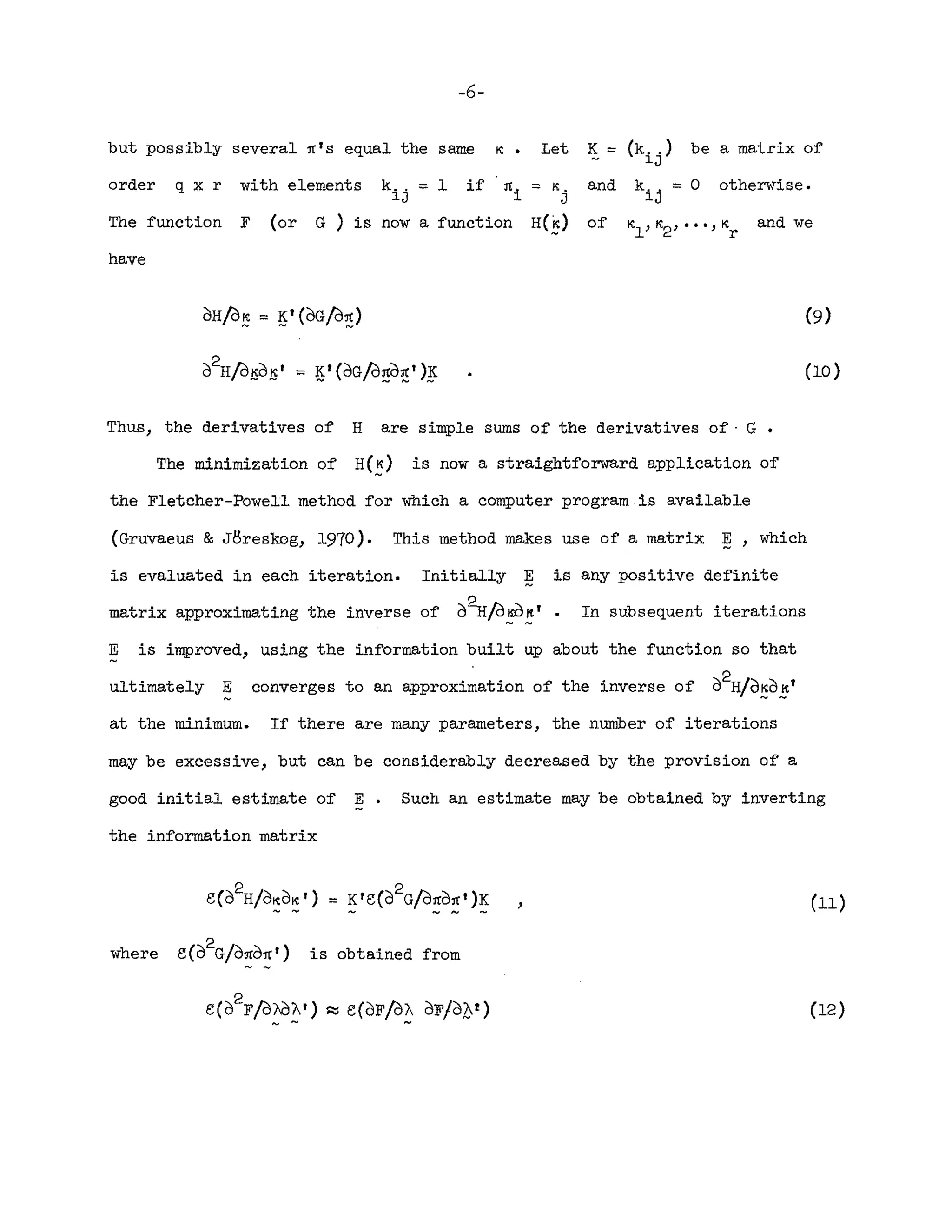
20. -18-
- b
1
(58)
This system may be estimated by the method of section 4.
To illustrate the application o~ the estimation procedure we use a
dispersion matrix S obtained ~rom ~ in (37) by subtracting the error
variances from the diagonal elements and deleting rows and columns corres-
ponding to C and Y. There are 6 nonf'Lxed elements in Band !',
These elements are functions of'
namely I3U
'
o~ the vector
1312 '
:rc •
1321 ) and These are the elements
and
b2 defined by [compare equation (31)]
1311
-1 0 0 0
1312
0 -1 0 0 a
l
1321
0 0 -1 0 a
2
1
::: + (39)
1322
0 0 -1 0 b
l
0
0 0 1 0 b
2
0 0 0 1
Thus the function F is a function o~ 4 independent parameters.
The function F was'minimized using only Fletcher-Powell iterations
starting from the point
The solution point, found after 8 iterations, was, as expected, a
l
= 0.8 ,
a
2
::: 0.4) b
l
= 0·3, b
2:::
0.2 with

21. A (0.2
1jr*=
0.1
0.1)
0·3
-19-
I~I = 0.05
6. An Economic Application
In this section we apply methods SFLGRV and RFLGRV to a small economic
model taken from the literature. The model is Klein's model of United
States economy presented in Klein (1950, Pl'. 58-66):
C == aO + alP + a2P_l + a,w + ~
I == bO + blP + b2P_l + b
3K_l
+ u
2
W* == Co + clE + c2E_l + c
3A
+ u:;
Y + T == C + I + G
Consumption:
Investment:
Private wages:
Product:
Income:
Capital:
Wages:
Private product:
y=p+w
K == K_l + I
w==W*+W**
E=Y+T-W** ,
(40a)
(40b)
(40c)
(40d)
(40e)
(40f)
(J+Og )
(40h)
where the endogenous variables are
C == consumption
I == investment
~. == private wage bill
P == profits
Y == national income
K = end-of-year capital stock
W == total wage bill
E = private product

22. -20-
and the predetermined variables are the lagged endogenous variables P-l,
K_
l
and E_
l
and the exogenous variables
1 ::: unity
W** == government wage bill
T indirect taxes
G == government expenditures
A = time in years :from 1931.
All variables except 1 and A are in billions of 1934 dollars.
This model contains eight dependent variables and eight predetermined
variables. There are three equations involving residual terms. The other
five equations are identities. Using the five identities (40d) - (40h),
P, Y, K, W and E may be solved for and substituted into (40a) -
(40c). This gives a model with the following structural form
C
- a - a a
l
- ~)
(:)
1 1
- b 1 - b b
l
1 1
- c - c 1
1 1
1
T
(0 a
3
- a -a a
1
0 a
2
0
~j
G
1 1
:::: b
O
- b -b b
l
0 b
2
b
3
A (41)
1 1
Co - c 0 c
1 c
3
0 0 P-l
1
K_l
E_l
There are 24 nonfixed elements in B and r . These are all linear
~
functions of the 12 unknown coefficients in (40a-c) as follows

23. -21-
1311
0 -1 0 0 0 0 0 0 0 0 0 0 1
(312 0 -1 0 0 0 0 0 0 0 0 0 0 0
(313 0 1 0 -1 0 0 0 0 0 0 0 0 0
1321
0 0 0 0 0 -1 0 0 0 0 0 0 0
(322 0 0 0 0 0 -1 0 0 0 0 0 0 rao 1
1323
0 0 0 0 0 1 0 0 0 0 0 0 0
a
1
(331 0 0 0 0 0 0 0 0 0 -1 0 0 0
(332 0 0 0 0 0 0 0 0 0 -1 0 0
a
2 0
r11
1 0 0 0 0 0 0 0 0 0 0 0 a
3
0
r12
0 -1 0 1 0 0 0 0 0 0 0 0
b
O
0
r13
0 -1 0 0 0 0 0 0 0 0 0 0 0
714 = 0 1 0 0 0 0 0 0 0 0 0 0
b
1 + 0 (42)
r16 0 0 1 0 0 0 0 0 0 0 0 0 b
2
0
r21
0 0 0 0 1 0 0 0 0 0 0 0
b
3
0
722
0 0 0 0 0 -1 0 0 0 0 0 0 0
723
0 0 0 0 0 -1 0 0 0 0 0 0 Co 0
724 0 0 0 0 0 1 0 0 0 0 0 0 c
1
0
726 0 0 0 0 0 0 1 0 0 0 0 0 0
c2
727
0 0 0 0 0 0 0 1 0 0 0 0 0
r31
0 0 0 0 0 0 0 0 1 0 0 0
C
3 0
r32 0 0 0 0 0 0 0 0 0 -1 0 0 0
r34 0 0 0 0 0 0 0 0 0 1 0 0 0
r35
0 0 0 0 0 0 0 0 0 0 0 11 0
r38 0 0 0 0 0 0 0 0 0 0 1 OJ 0
From annual observations, United States, 1921-1941 the f'o11owing raw
moment matrices are obtained:
C I W*-
e (62166063
28560086)
S = I 1679,01 286.02
~yy
W* 42076.78 1217·92

24. -22-
C I W*
1 1133·90 26.60 763.fJJ
W** 5977·33 103.80 4044.07
T 7858.86 160 .40 5315·62
G 11633.68 243.19 7922.46
s =
A 577·70 -105.60 460·90
-xy
P-1 18929·37 655·33 12871·73
K_1 227767·38 5073·25 153470·56
E_1 66815·25 1831.13 45288·51
1 W** T G A P K_
1
E_
1
1 21.00 -1
W** 107·50 626.87
T 142·90 789·27 1054·95
G 208.20 1200.19 1546.11 2369·94
s = 238.00 176.00 421·70
-ocx A 0.00 770.00
P-1 343·90 1746~22 2348.48 3451.86 -11·90 5956.29
K_
1 4210.40 21683.18 28766.23 42026.14 590.60 69073·54 846132·70
E_1 1217·70 6364.43 8436·53 12473·50 495·60 20542.22 244984·77 72200.03
The ~o11owing estimated model was obtained
with
C = 18.318 - 0.229P + 0.384p + 0.802W + u "1",
-1 1
I = 27·278 - 0·797P + 1.051P_1 - 0.l48K_1 + ~ I
W* = 5·766 + 0.235E + 0.284E_1 + 0.234A + ~ .~
(43)
(44)

25. -23-
The standard errors of the estimated parameters may be obtained from a
formula for the asymptotic variance-covariance matrix developed by Rothenberg
and Leenders (1964).
7. The Special Case of No Residuals
When there are no residuals in (1), the relations between ~ and ~
are exact. The joint distribution of ~ and ~ is singular and of rank n •
vanishes. In general)
and r or in ~ e
-5
and e ) this model has to be estimated by the method of section 3. This
~E
In the equation (4) for ~ ) the second term in ~
-yy
when there are fixed and constrained elements in B
may be done by choosing 0/ = 0 and specifying the fixed elements and the
constraints as described in that section.
The matrix ~ can also be written
,
where
e = (~E Q) ,
Q ~5
(46)
from which it is seen that the model is identical to a certain restricted
factor analysis model. Several special cases will ~ow be considered.
If B = I and r is unconstrained, i.e., all elements of r are
- -
regarded as free parameters, model (45) is formally equivalent to an un-
restricted factor model (JClreskog, 1969). The matrix i. in (46) may be
obtained from any 0* of order (m + n) x n satisfying

26. -24-
2
r. == 11.*/1,*' + e
by a transformation of 11.* to a reference variables solution where the x's
are used as reference variables. Maximum likelihood estimates of 11.* and e
may be obtained by the method of JBreskog (1967a,b) which also yields a large
sample x
2
test of goodness of fit. Let the estimate of 11.* be partitioned
as
, (48)
where is of order m x n and ~ of order n x n • Then the maximum
likelihood estimates of r and ~ are
(50 )
If B == I and r is constrained to have some fixed elements while the
remaining elements in r are free parameters, model (45) is formally equiva-
lent to a restricted factor model in the sense of JBreskog (1969). This model
may be estimated by the procedure described in the same paper and, in large
samples, standard errors of the estimates and a goodness of fit test can also
be obtained. A computer program for this procedure is available (JBreskog &
Gruvaeus, 1967).
A more general case is when B is lower triangular. The structural
equation system for the true variates is then a causal chain. In general
such a causal chain may be estimated by the method described in section 3

27. -25-
of the paper, though there may be simpler methods. One example occurs when
the system is normalized by fixing one element in each row of r to unity
and B has the form
B :
o
1322
o
••• 0
where all the I3ls are free parameters. Then there is a one-to-one trans-
formation between the free parameters of B and the free elements of
A : B-1• One may therefore estimate A instead of B. In this case,
the variance-covariance matrix ~ is of the form
where
Model (51) is a special case of a general model for covariance structures
developed by J8reskog (1970) and may be estimated using the computer program
ACOVS (J8reskog, Gruvaeus & van Thillo, 1970). In this model £, 1?
and e may contain fixed parameters and even parameters constrained to be
-€
equal in groups. The computer program gives maximum likelihood estimates of
the free parameters in ~, r , and, in large samples,
standard errors of these estimates and a test of overall goodness of fit of
the model can also be obtained.

28. -26-
More generally, the above mentioned method may be used whenever ~
can be written in the form (51) such that there is a one-to-one correspondence
between the free parameters in Band r and the distinct free elements in
B* and A. For a less trivial example, see J8reskog (1970, .section 2.6).
8. A Psychological Application
In this section we consider a simplified model for the prediction of
achievements in mathematics (M) and science (S) at different grade levels.
To estimate the model we make use of longitudinal data from a growth study
conducted at Educational Testing Service (Anderson &Maier, 1963; Hilton,
1969). In this study a nationwide sample of fifth graders was tested in
1961 and then again in 1963, 1965 and 1967 as seventh, ninth and eleventh
graders, respectively. The test scores employed in this model are the
verbal (V) and quantitative (Q) parts of SCAT (Scholastic Aptitude
Test) obtained in 1961 and the achievement tests in mathematics (M5,~,M9'
M
l l
) and science (S5,S7,8
9,Sll)
obtained in 1961, 1963, 1965, and 1967,
respectively. The achievement tests have been scaled so that the unit of
measurement is approximately the same at all grade levels.
The model is depicted in Figure 1, where V
M
l l
, 8
5
,
~l' S2' •• " ~8
is
8
7
, 8
9
and 8
11
denote the true scores of the tests and
the corresponding residuals. The model for the true scores
(53a)
(53b)

29. -27-
This model postulates the major influences of a student's achievement in
mathematics and science at various grade levels. At grade 5 the main
determinants of a student 's achievements are his verbal and quantitative
(53c)
(53d)
(53e)
(53g)
(53h)
abilities at that stage. At higher grade levels, however, the achievements
are mainly determined by his achievements in the earlier grades. Thus,
achievements in mathematics in grade i is determined mainly by the
achievements in mathematics in grade i - 2 , whereas achievements in sci-
ence in grade i is determined mainly by the achievements in science in
grade i - 2 and in mathematics in grade i, i = 7,9,11 •
The structural form of this model is
1 0 0 0 0 0 0 0 M
5
a
1
a
2 Sl
0 "I 0 0 0 0 0 0 8
5
b
l
b
2 s2
-c 0 1 0 0 0 0 0
~
0 0 S3
1
0 -d -d 1 0 0 0 0 8
7
0 0
(:) +
S4
1 2 =
0 0 -e 0 1 0 0 0 M
9
0 0
S5
1
0 0 0 -f -f 1 0 0 8
9
0 0 S6
1 2
0 0 0 0 -gl 0 1 0 MIl 0 o I S7
0 0 0 0 0 -hI -h 8
11
0 o I Sa
2 J

30. -28-
It is seen that this model is a causal chain. The model can be estimated by
the method described in section 5, provided some assumption is made about the
intercorrelations of residuals Sl'S2' ••• 'S8. Without such an assumption
the model is not identified. We have chosen to make the assumption that
all residuals are uncorrelated except Sl and S2· This assumption does
not seem to be too unrealistic.
The data that we use consist of a random sample of 730 boys taken from
all the boys that took all tests at all occasions. The variance-covariance
matrices are
M
5
130.690
115·645
116.162
90·709
119·564
104.430
119·712
90·916
179·617
125.858·
114.364
l25·223
135·074
126.470
116·950
193·557
120.426
155·885
157.827
149·930
117.439
148.648
120.492
133·231
112.218
109·187
215·894
159·783
175·497
155.839
218.067
149·045
147.115
264.071
143·218 190.763
,
~
106.837
87·859
8
9
107.75°
72·534
MIl
107·042
89·617
,
v
s = V (.158.014
~xx Q 73.518
The estimated model is
~ "= o.64ov + 0.415Q + ~1 (55a)
(55b)
(55c)

31. -29-
8
7
= 0.3258
5 + 0.493M7 + ~4
M
9
= 1.027M7 + ~5
(55d)
(55e)
(55f)
(55g)
(55h)
The estimated variance-covariance matrix of the true scores V and Q is
V
A V (105048
(l> = Q 73.95
Estimated residual variances and error variances for each measure are given
below
Measure
V
Q
M
5
8
5
M
7
8
7
M
9
8
9
M
l l
811
Residual Variance
10.0
22·5
26.4
29·5
25·2
28·5
75·7
20.0
Error Variance
}?l
4.4
25.4
11.8
40·3 .
24.3
29·3
36.1
18.8
47.7

32. -30-
The estimated correlation between ~l and ~2 is 0.17·
The estimated reduced form for the true scores is
M = 0.640v + 0.415Q + ~*
5 1
~ = 0·70211 + 0.455Q + ~3
M
9
= 0·721V + 0.467Q + ~5
8
9
= 0.815V + 0.296Q + ~6
8
11 = 0.663V + 0.277Q + ~8
The relative variance contributions of V and Q, the residual ~* and
the error, to each test's total variance are shown below:
Measure V and Q Residual Error
M
5
0·73 0.08 0.19
8
5
0.78 0.15 0.07
~ 0·59 0.20 0.21
8
7 0·56 0.28 0.16
M
9
0·56 0.30 0.14
8
9
0·52 0.32 0.16
M
l l
0.42 0·51 0.07
8
11 0.42 0·33 0.25
(56a)
(56c)
(56e)
(56f)
(56g)
(56h)

33. -31-
It is not easy to give a clear-cut interpretation of these results.
Inspecting first the equations (55c), (55e) and (55g), it is seen that.a
unit increase in M. 2 tends to have a smaller effect on M. the larger
1.- 1.
i is. This agrees with the· fact that the growth curves in mathematics
"flattens" out at the higher grade levels. One would expect that the co-
efficient in (55g), like in (55c) and el in (55e), would be
greater than one, since, in general, for these data, the correlation of status,
M. - M. 2 ' are positive although usually very small.
1. 1.-
However, the large residual variance ~7 suggests that M
9
alone is not
sufficient to account for M
l l•
This is probably due to the fact that
mathematics courses at the higher grades change character from being
mainly Itarithemetic computation" to involving more "algebraic reasoning."
Inspecting next the equations (55d), (55f) and (55h) describing
science achievements, it is Seen that the influence of mathematics on
science tends to decrease at the higher grades. This is natural since
science courses in the lower grades are based mainly on "logical reasoning"
whereas in the higher grades they are based on "m
emorizing of facts. It The
effect of science achievements on science two years later first increases
and then decreases. This is probably because the science courses special-
ize into different courses (Biology, Physics, etc.) at grade 11 whereas
the science test at the lower grades measures some kind of overall 11science
knowledge."
Whatever may be the best interpretations of these results, the example
serves to illustrate that it is possible to have both errors in equations
and errors in variables and still have an estimable model.

34. -32-
References
Anderson, T. W. An introduction to multivariate statistical analysis. New
York: Wiley, 1958.
Anderson, S. B., &Maier, M. H. 34,000 pupils and how they grew. Journal
of Teacher Education, 1963, ~ 212-216.
Blalock, H. M. Causal inferences in nonexperimental research. Chapel Hill,
N. C.: University of North Carolina Press, 1964.
Brown, T. M. Simplified full maximum likelihood and comparative structural
estimates. Econometrica, 1959, g]j 638-653.
Brown, T. M. Simultaneous least squares: a distribution free method of
equation system structure estimation. International Economic Review,
1960, b 173-191.
Chernoff, H., & Divinsky, N. The computation of maximum-likelihood estimates
of linear structural equations. In W. C. Hood & T. C. Koopmans (Eds.),
Studies in econometric method, Cowles Commission Monograph 14. New York:
Wiley, 1953. pp. 236-269.
Chow, G. C. Two methods of computing full-information maximum likelihOod
estimates in simultaneous stochastic equations. International Economic
Review, 1968, 2." 100-112.
Eisenpress, H. Note on the computation of full-information maximum-likelihood
estimates of coefficients of a simultaneous system. Econometrica, 1962,
2£, 343-348.
Eisenpress, H., & Greenstadt, J. The estimation of non-linear econometric
systems. Econometrica, 1966, ~ 851-861.

35. -33-
Fletcher, R., & Powell, M. J. D. A rapidly convergent descent method ~or
minimization. The Computer Journal, 1963, £, 163-168.
Goldberger, A. S. Econometric theory. New York: Wiley, 1964.
Gruvaeus, G., &J8reskog, K. G. A comPuter program for minimizing a function
o~ several variables. Research Bulletin 70-14. Princeton, N. J.:
Educational Testing Service, 1970.
Hilton, T. L. Growth study annotated bibliography. Progress Report 69-11.
Princeton, N. J.: Educational Testing Service, 1969.
Johnston, J. Econometric methods. New York: McGraw-Hill, 1963.
J8reskog, K. G. Some contributions to maximum likelihood factor analysis.
Psychometrika, 1967, ~ 443-482. (a)
J8reskog, K. G. UMLFA--A computer program for unrestricted maximum likelihood
~actor analysis. Research Memorandum 66-20. Princeton, N. J.: Educational
Testing Service, revised edition, 1967. (b)
J8reskog, K. G. A general approach to confirmatory maximum likelihood factor
analysis. Psychometrika, 1969, ~ 183-202.
J8reskog, K. G. A general method for analysis of covariance structures.
Biometrika.. 1970, 2L 239-251-
J8reskog, K. G., & Gruvaeus, G. RMLFA--A computer program for restricted
maximum likelihood factor analysis. Research Memorandum 67-21. Princeton:
N. J.: Educational Testing Service, 1967.
J8reskog, K. G., Gruvaeus, G. T., & van Thil1o, M. ACfJVS--A general computer
program ~or analysis of covariance structures. Research Bulletin 70-15.
Princeton, N. J.: Educational Testing Service, 1970.

36. -34-
JBreskog, K. G., & van Thill0, M. LISREL--A general computer program for
estimating linear structural relationships. Research Bulletin 70-00.
Princeton, N. J.: Educational Testing Service, in preparation.
Klein, L. R. Economic fluctuations in the United States, 1921-1941, Cowles
Commission Monograph 11. New York: Wiley, 1950.
Klein, L. R. A textbook of econometrics. Evanston: Row, Peterson, 1953.
Klein, L. R. Estimation of interdependent systems in macroeconometrics.
Econometrica, 1969, 2L 171-192.
Koopmans , T. C., Rubin, H., & Leipnik, R. B. Measuring the equation systems
of dynamic economics. In T. C. Koopmans (Ed.), Statistical inference
in dynamic economic models, Cowles Commission Monograph 10. New York:
Wiley, 1950. pp. 53-237·
Malinvaud, E. Statistical methods of econometrics. Chicago: Rand-McNally,
1966.
Rothenberg, T. G., & Leenders, C. T. Efficient estimation of simultaneous
equation systems. Econometrica, 1964, 32, 57-76.
Turner, M. E., & Stevens, C. D. The regression analysis of causal paths.
Biometrics, 1959, Q, 236-258·
Wegge, L. L. A family of functional iterations and the solution of maximum
likelihood estimation equations. Econometrica, 1969, 2L 122-130.
Werts, C. E., & Linn, R. L. Path analysis: Psychological examples.
Psychological Bulletin, 1970, Ii (3), 193-212.
Wold, H., & Jureen, L. Demand analysis. New York: Wiley, 1953.
Zellner, A. An efficient method of estimating seemingly unrelated
regressions and tests for aggregation bias. Journal of the
American Statistical Association, 1962, 21, 348-368.

37. -35-
A. Appendices of Mathematical Derivations
Al. Matrix Derivatives of Function F in Section 3
The function is
(Al)
which is regarded as a function of B, r, ~, ~, ~o' ~E defined by
(4). To derive the matrix derivatives we shall make u£e of matrix dif-
ferentials. In general, dX = (dx
i j
) will denote a matrix of differentials
and if F is a function of X and dF = tr(Q~t) then dF/d~ = Q •
-1 1
Writing A = Band Q== ~- r = AI' we have
= Adf' - AdBAr
== Adf' - AdBD
Furthermore, since in general,
(A2)
(A3)
and
dlog Ixl

38. -36-
we obtain from (Al),
(A4)
where n is defined by (12) and dE is partitioned the same way as n in
(12) .
From (~-) and the def'initicns of' A and D we have
z :::: DPDf + ~'k~t
2
+ e
-yy -€
L. :::: r;' :::: ~:QI
-xy -yx
L. ::::
~ + r£<}
-xx -5
(A5)
(A6)
from which we obtain
dL. :::: D~dD' + Dd~D' + dD~D'
-yy
+ A'VdAt + Ad1jrA' + dA1jrAI
+ 213 de
_E ~e
(AB)
(A10)

39. -37-
Substitution of dA and dD from (A2) and (A3) into (AB) and (A9)
gives
+ AdI1!D' - AdB])1lD'
- A"ljrA'dB'A' - AdBA1jfAt
+ Dd<PD' + Ad1jfA' + 2e de
. -€ -€
, (All)
c1>D rdB'A' + d<!JDt (A12)
Substitution of (All), (A12) and (AIO) into (A4), noting that tr(CtdX)
= tr(~rg) = tr(2~t) and collecting terms, shows that the matrices multiplying
d!lt, dr', d~, dljr, d~8 and d@€ are the matrices on the right sides of
equations (14), (15), (17), (18) and (19) respectively. These are therefore
the corresponding matrix derivatives.
A2. Information Matrix for the General Model of Section 3
In this section we shall prove a general theorem concerning the expected
second-order derivatives of any function of the type (8) and show how this
theorem can be applied to compute all the elements of the information matrix
(12).
We first prove the following
N
Lemma: Let S = (liN) ~l (~a - ~)( ~a - ~) r ). where ~l' ~2' ••• , ~N are
independently distributed according to N(~,~). Then the asymptotic

40. -38-
distribution of the elements of n = E-l(E - S)~-l is multivariate
..... ..... -- ......-
normal with means zero and variances and covariances given by
(A13)
Proof: The proof follows immediately by multiplying w~ = E E ~ag(~gh - Sgh)~h~
. . g h
and w = E E ~l(~.. - s .. )crJ V and using the fact that the asymptotic vari-
I-J.V .. lJ lJ .
1 J
ances and covariances of S are given by
Ne [(cr h - s h)(cr.. - s . .)]
g g lJ lJ
(see e.g., Anderson, Theorem 4.2.4).
IT .~ • + C1 ~
gl hJ gj hi
We can now prove the following general theorem.
Theorem: Under the conditions of the above lemma let the elements of E be
functions of two parameter matrices ~ = (I-J.
gh
) and N = (Vi j
)
let F(~,~) = ~ N[logl~1 + tr(§~-l)] with OF/O~ = NAnB and
OF/O~ = N~p. Then we have asymptotically
and
( / ) ( ,2 ,I " ) -1) ( -1) ( ~'"-In) . (B! E-Ie! )h' . ( 4)
1 Ned 11) OI-J. hOv.. =(IV:, e I • B!E D h' + ~ Al
g lJ gl J gJ ].
Proof: Writing OF/OI-J.gh = Na~p)O:p'bAh and OF/Ov .. = Nc, w d . , where it
g..;:. I f-' f-' lJ ljl I-J.V YJ
is assumed that every repeated subscript is to be summed over, we have
2
(I/N)e(o F/Ojl hOY .. ) = (l/N)e(OF/OI-J. hOF/Ov.. )
g lJ g lJ
= N e(a~P)NAbA~c. w d j)
g..;:. ~ pr; au I-J.v V
= N a~bAhc. d .e(w~w )
o~ f-' ll-J. vJ "'1-" I-J.v

41. -39-
It should be noted that the theorem is quite general in that both M
and N may be row or column vectors or scalars and M and N may be
identical in which case, of course, ~ ~ 9 and B =D •
We now show how the above theorem can be applied repeatedly to compute
all the elements of the information matrix (12). To do so we write the
derivatives (14) - (19) in the form required by the theorem.
Let A ~ B-1 and ~ ~ ~-l~ , as before, and
T[m x (m + n)] ~ [A' 0]
P[(m + n) x m] ~~~' + ~!~J
<PD'
Q[(m + n) x n]
.(;)
~[(m + n) x n] • G)
Then it is readily verified that
dF/OB ~ -NT.I1P
dF/dr ~ NT.I1Q
dF/d(J) = NR'.I1R
(A15)
(Al6)
(A18)
(A20)
(A21)
(A22)

42. -40-
dF/d8 :::: Nne (A23)
In the last equation we have combined (18) and (19) using 8 ::::~o 9.
- ~ 8J
A3. Matrix Derivatives of Funct:i,on F in Section 4
The function is defined by
,
where
One finds immediately that
( -1 ) -1 )
dF :::: tr ~ d~ - 2tr(B dB
"'" "'" -"....
:::: tr[~-l(dBS Bt + BS dB' - dES r t - rs dB')]
- ~~YY- --yy - ~-yx- --x:y-.' ~
-1
- 2tr(!? d~)
,
so that the derivatives dFf2JB and dFf2Jr are those given by (29) and
- ~
()O ).

43. Sl
S2
~3
~
8
7
~
~
4
S5
M
9
8
9
S6
S7
M
l
1
8
n
i"
"8
I
+:-
f-1
I
Fig.
1.
Model
for
Achievements
in
Mathematics
and
Science