SlideShare a Scribd company logo
Newsletter 20
1
: How can we deal with big data set comprised of several thousand
DMUs?
: You can divide them into several groups consisting of a few
hundred DMUs and solve each group for finding efficient DMUs in the
group. Then, merge the efficient DMUs into one set. Solve the set and
find the final efficient DMUs. Using the finalist, re-evaluate each group.
Version 16.0: Desirable Inputs Model
Generally speaking, in DEA, inputs (I) indicate input resources and
the smaller the better, while outputs (O) correspond to productions
induced by inputs (I), which are the larger the better. Among outputs,
there exist undesirable outputs (OBad) incidental to outputs, e.g. CO2,
which are the smaller the better. In this version, we propose a new
input style, called Desirable inputs (IGood), which are the larger the
better. We show four potential examples of (IGood).
(a)In accordance with the increasing concern on environmental
pollution, spread of Electric cars is worldwide required. We
compare the energy consumption issue of countries. We consider
“Number of Electric Cars” as a Good Input (IGood). Other IO items
are (I) Total consumption of Energy, (O) GDP and (OBad)
Pollutants (e.g. CO2). DMUs are Country 1 to Country N.
(b)We consider the case that there are many new projects in a
company and the manager wishes to evaluate the efficiency of
projects. For this purpose, a certain number of evaluators is
assigned to each project and they report Cost (Input), Return
DEA-Solver-Pro Newsletter
No. 20
(Jan 7, 2022)
Newsletter 20
2
(Output), Risk (Undesirable Output) for the assigned project. In this
case, we consider the number of evaluators is a Desirable input
(IGood) and the larger the better.
(c)We point to “Women’s Rights Movements” in a country where
women’s right is not fully guaranteed. In such a country, suppose
local governments where men and women are serving as officers.
They are inputs to office, while women are (IGood) and men are
(I). As outputs, we assume (O) Service and (OBad) Claims.
(d)Suppose that, inspired by COVID-19, many medical enterprises
are eager to develop vaccine. In this case, (IGood) Number of test
takers, (I) Cost, (O) Recovery, (OBad) Failure. As DMUs, we
assume potential Vaccine1 to Vaccine N.
We reasoned that such situations occur in many fields of enterprise.
We formulate this situation in the framework of SBM.
In Version 15.1, we added the CRS (constant returns-to-scale)
version to NegativeData_SBM models. Furthermore, as for Malmquist
models, we added the cumulative and the adjusted Malmquist indices.
In DEA, we often encounter negative data, e.g. financial data. In
response to many requests, in this Version 15.0, we updated SBM
models to cope with negative data. Three clusters are added under
the Variable Returns-to-Scale (VRS) model. They are (1)
NegativeData_SBM, (2) NegativeData_SBM_Max and (3)
NegativeData_Malmquist. Now, we can deal with positive and
negative data in a single model. The efficiency scores are units
invariant and translation invariant.
Newsletter 20
3
In Version 14.0, we introduced SBM_Bounded models as an
extension of the SBM_Max models. In real world applications, there
are cases where input-reduction and/or output expansion are
restricted by some external constraints. For example, suppose that
expansion of inpatient visits, as an output of hospitals, is bounded by
3% of the current value due to physical environments. Input reduction
bound and output expansion bound differ for every input and every
output. The SBM_Bounded models handle these cases as the
constraints to slacks which are obtained by SBM_Max models. Hence,
the projection of inefficient DMUs thus obtained indicates more
practical and useful improvement (Kaizen) plan. In Figure 14.0, we
illustrate the model in the input side projection. DMUs A, B, C and D
are on the efficient frontier while P and S are inefficient. P will be
projected to R by the SBM_Max model, whereas the bounded area
forces it to stop at Q. The bounded area is determined by Input 1
reduction rate and Input 2 reduction rate which are assumed to be
common to all DMUs. DMU S is projected to T inside its bounded area
and on the efficient frontier.
Input 1
Input 2
A
B
C
D
●P
● Q
●S
T ●
R
0
Newsletter 20
4
Figure 14.0: SBM_Bounded model
In Version 14.0, we have revised the SBM_Max models.
In Version 13.2, we added Super-Efficiency score to the SBM_Max
model.
In Version 13.0, we replaced SBM_Variation models in the earlier
version by SBM_Max models. The SBM models usually report the
worst efficiency scores for inefficient DMUs. This means that the
projected point is the farthest one on the associated efficient frontier.
In contrast, SBM_Max models look for the nearest point on the
associated efficient frontier. Hence, the efficiency score is, in a sense,
maximized as contrasted to the ordinary SBM (Min) models. This
indicates that we can attain an efficient status with less input
reductions and less output expansions than the ordinary SBM (Min)
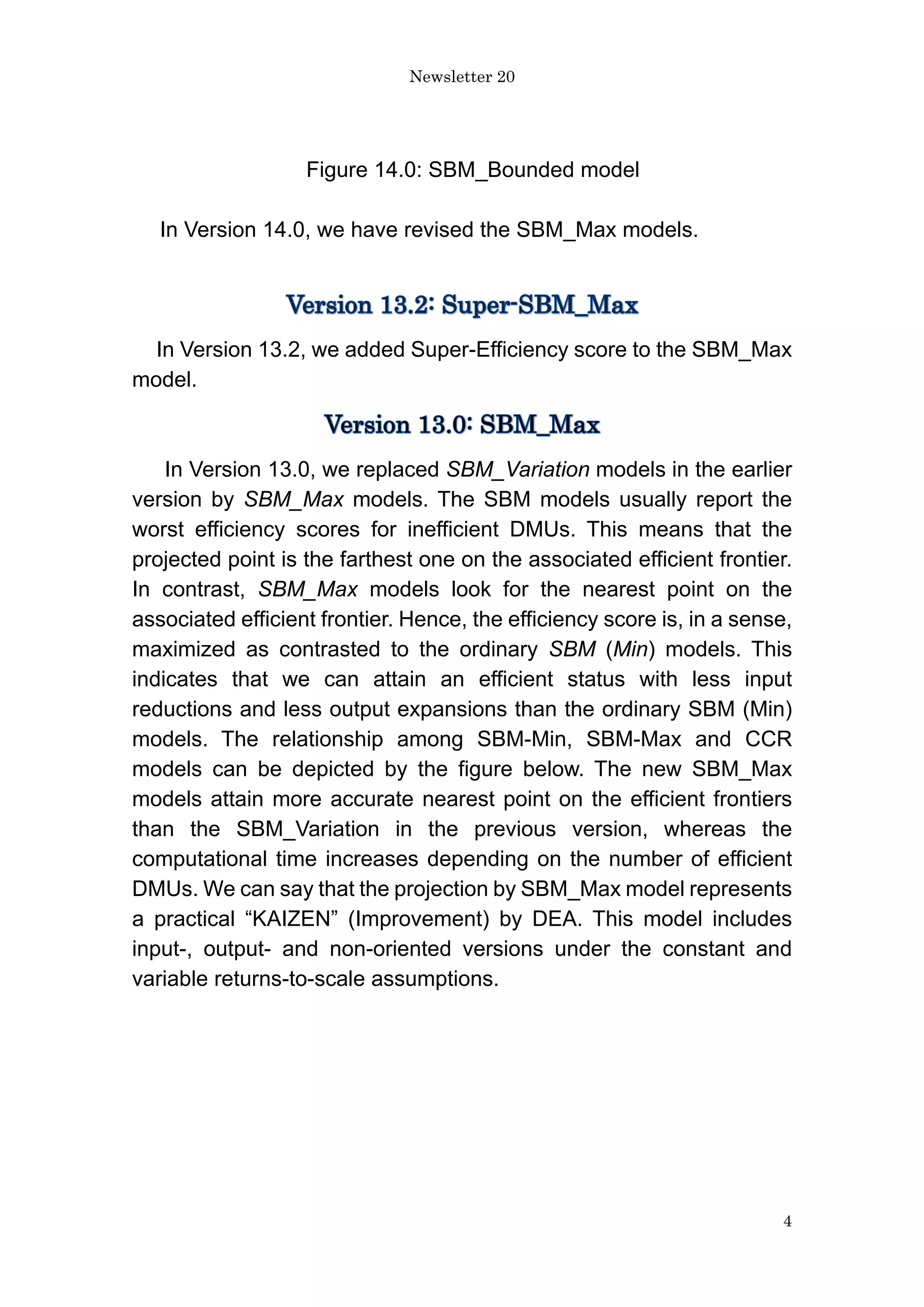
models. The relationship among SBM-Min, SBM-Max and CCR
models can be depicted by the figure below. The new SBM_Max
models attain more accurate nearest point on the efficient frontiers
than the SBM_Variation in the previous version, whereas the
computational time increases depending on the number of efficient
DMUs. We can say that the projection by SBM_Max model represents
a practical “KAIZEN” (Improvement) by DEA. This model includes
input-, output- and non-oriented versions under the constant and
variable returns-to-scale assumptions.
Newsletter 20
5
Figure 13.1: SBM-Min, CCR and SBM-Max
In Version 12.0, we introduced Directional Distance (Function)
Model that computes the efficiency of DMUs along the given direction.
We offer two types of efficiency, i.e., ordinary and super efficiency.
The Directional Distance model (DD model) has three variations: (1)
Input- (2) Output- and (3) Non-oriented. Each variation has two
returns-to-scale (RTS): (a) CRS (Constant RTS) and (b) VRS
(Variable RTS).
The DD model deals with two kinds of input and three kinds of output
as follows.
(a)Directional (Ordinary) inputs (I)
The heading of this class is (I) and its value is denoted by
( )
( 1, , ; 1, , )
I
ij
x i I j n
= =
  where 1, ,
i I
=  corresponds to input and 1, ,
j n
= 
indicates DMU. The component of directional vector is defined as
( ) ( )
I I
ij ij
d x
= .
Input 1
Input 2
O
Newsletter 20
6
(b)Non-directional inputs (IN)
The heading of this class is (IN) and denoted by ( )
( 1, , ; 1, , )
IN
ij
x i IN j n
= =
 
where IN is the number of (IN) inputs. The component of directional
vector is defined as ( )
0
IN
ij
d = . This class has no directional effect on the
efficiency score, but associates with it through the intensity vector.
This class is the secondary input and can be empty.
(c)Directional (Good) output (O)
The heading of this class is (O) and denoted by ( )
( 1, ,O; 1, , )
O
ij
y i j n
= =
 
where O is the number of good outputs. The component of directional
vector is defined as ( ) ( )
O O
ij ij
d y
= .
(d)Non-directional outputs (ON)
The heading of this class is (ON) and denoted by
( )
( 1, ,ON; 1, , )
ON
ij
y i j n
= =
  where ON is the number of non-directional
outputs. The component of directional vector is defined as ( )
0
ON
ij
d = .
This class has no directional effect on the efficiency score, but
associates with it through the intensity vector. This class is the
secondary output and can be empty.
(e)Undesirable outputs (OBad)
The heading of this class is (OBad) and denoted by
( )
( 1, ,OBad; 1, , )
OBad
ij
y i j n
= =
  where OBad is the number of undesirable
outputs. The component of directional vector is defined as
( ) ( )
OBad OBad
ij ij
d y
= . This class can be empty.
In Version 11.0, we introduced a new model called “Resampling in
DEA”. This model deals with data variations and gives confidence
Newsletter 20
7
intervals of DEA scores. Input/output values are subject to change for
several reasons, e.g., measurement errors, hysteretic factors,
arbitrariness and so on. Furthermore, these variations differ in their
input/output items and their decision-making units (DMU). Hence,
DEA efficiency scores need to be examined by considering these
factors. Resampling based on these variations is necessary for
gauging the confidence interval of DEA scores. We propose four
resampling models. The first one assumes downside and upside
measurement error rates for each input/output, which are common to
all DMUs. We resample data following the triangular distribution that
the downside and upside errors indicate around the observed data.
The second model evaluates the downside and upside error rates
from historical data. The third model utilizes historical data, e.g., past-
present, for estimating data variations, imposing chronological order
weights which are supplied by Lucas series (a variant of Fibonacci
series). This model provides different downside and upside error rates
for each DMU. The last one deals with future prospects. This model
aims at forecasting the future efficiency score and its confidence
interval for each DMU. Table 11.1 exhibits a sample of forecast DEA
scores and their confidence intervals, while Figure 11.1 shows 95%
confidence interval of forecast scores.
Table 11.1: Forecast DEA score and confidence interval
DMU Forecast 97.50% 90% 80% 75% 50% 25% 20% 10% 2.50%
H1 0.946 1.122 1.092 1.062 1.036 0.925 0.880 0.870 0.849 0.818
H2 1.043 1.128 1.098 1.079 1.073 1.049 0.906 0.883 0.845 0.815
H3 0.708 0.743 0.722 0.709 0.704 0.683 0.662 0.657 0.645 0.625
H4 0.809 0.828 0.809 0.796 0.792 0.769 0.747 0.742 0.728 0.708
H5 0.719 0.748 0.727 0.714 0.709 0.689 0.668 0.663 0.651 0.633
H6 1.067 1.185 1.146 1.124 1.115 1.084 1.055 1.049 1.033 0.993
H7 0.900 0.918 0.894 0.879 0.874 0.849 0.826 0.820 0.805 0.782
H8 0.795 0.877 0.835 0.809 0.798 0.762 0.730 0.722 0.705 0.680
H9 0.689 0.736 0.707 0.689 0.681 0.655 0.630 0.623 0.606 0.582
H10 0.801 1.065 0.981 0.914 0.891 0.791 0.748 0.740 0.720 0.689
H11 0.866 1.010 0.947 0.914 0.902 0.861 0.826 0.819 0.798 0.771
H12 1.013 1.014 0.992 0.961 0.951 0.911 0.878 0.870 0.850 0.822
Newsletter 20
8
Figure 11.1: Forecast DEA score and 95% confidence interval
In Version 10.0, we introduced the “Non-convex DEA” model. In
DEA, we are often puzzled by the large difference between the
constant-returns-scale (CRS) and variable returns-to-scale (VRS)
scores, and by the convexity production set syndrome in spite of the
S-shaped curve often observed in many real data sets. See Figure
10.1. In this model, we propose a solution to these problems.
0.000
0.200
0.400
0.600
0.800
1.000
1.200
1.400
H1 H2 H3 H4 H5 H6 H7 H8 H9 H10 H11 H12
97.50% DEA 2.50%
0
1
2
3
4
5
6
7
8
0 1 2 3 4 5 6 7 8 9 10 11
y
x
Newsletter 20
9
Figure 10.1: S-shaped data
In Version 9.0, we introduced a model called “DNSBM” (dynamic
SBM with network structure). We have already introduced the network
SBM (NSBM) and the dynamic SBM (DSBM) models separately.
Hence, this model is a composite of these two models. Vertically, we
deal with multiple divisions connected by links of network structure
within each period and, horizontally, we combine the network
structure by means of carry-over activities between two succeeding
periods. See Figure 9.1 below. This model can evaluate (1) the overall
efficiency over the observed entire period, (2) dynamic change of
period (term) efficiency (3) dynamic change of divisional efficiency
and (4) divisional Malmquist index. The model can be implemented in
input-, output- or non-(both) oriented forms under the CRS or VRS
assumptions on the production possibility set. We can impose the
initial condition on the carry-overs.
We can formally deal with bad carry-overs, such as nonperforming
loans and dead stock, in this model. We modified the data formats of
Dynamic SBM (DSBM) and Network SBM (NSBM) so that they are
compatible with DNSBM model. Please see User’s Guide Version
10.0.
Newsletter 20
10
Figure 9.1: Dynamic model with network structure
In Version 8.0 we introduced a model called “EBM” (epsilon-based
measure of efficiency) for measuring technical efficiency. DEA is a
data driven tool for measuring efficiency of decision making units
(DMU) and shows a sharp contrast to so-called “parametric methods”
such as stochastic frontier analysis (SFA). The latter methods assume
specific production function forms to be identified. This assumption is
not so reasonable in several instances and aspects. Since DEA can
deal with multiple inputs vs. multiple outputs relations in a single
framework, it is becoming a method of choice for efficiency evaluation.
However, DEA has several shortcomings to be explored further. In
DEA, we have two measures of technical efficiency with different
characteristics: radial and non-radial. Historically, the radial measure,
represented by the CCR model was the first DEA model, whereas the
non-radial model, represented by the SBM model was a latecomer.
For instance, in the input-oriented case, the CCR deals mainly with
proportionate reduction of input resources. In other words, if the
Carry- Over
Carry- Over
Carry- Over
Output
Output 2
Output 3
Division 2
Division 3
Division 1
Link 2→3
Link 1→2
Input 2
Division 2
Division 3
Division 1
Input 3
Input 1
Output 1
Output 2
Output 3
Link 2→3
Link 1→2
Input 2
Input 3
Period t
Input 1
Period t+1
Newsletter 20
11
organisational unit under study has two inputs, this model aims at
obtaining the maximum rate of reduction with the same proportion, i.e.
a radial contraction in the two inputs that can produce the current
outputs. In contrast, the non-radial models put aside the assumption
of proportionate contraction in inputs and aim at obtaining maximum
rates of reduction in inputs that may discard varying proportions of
original input resources.
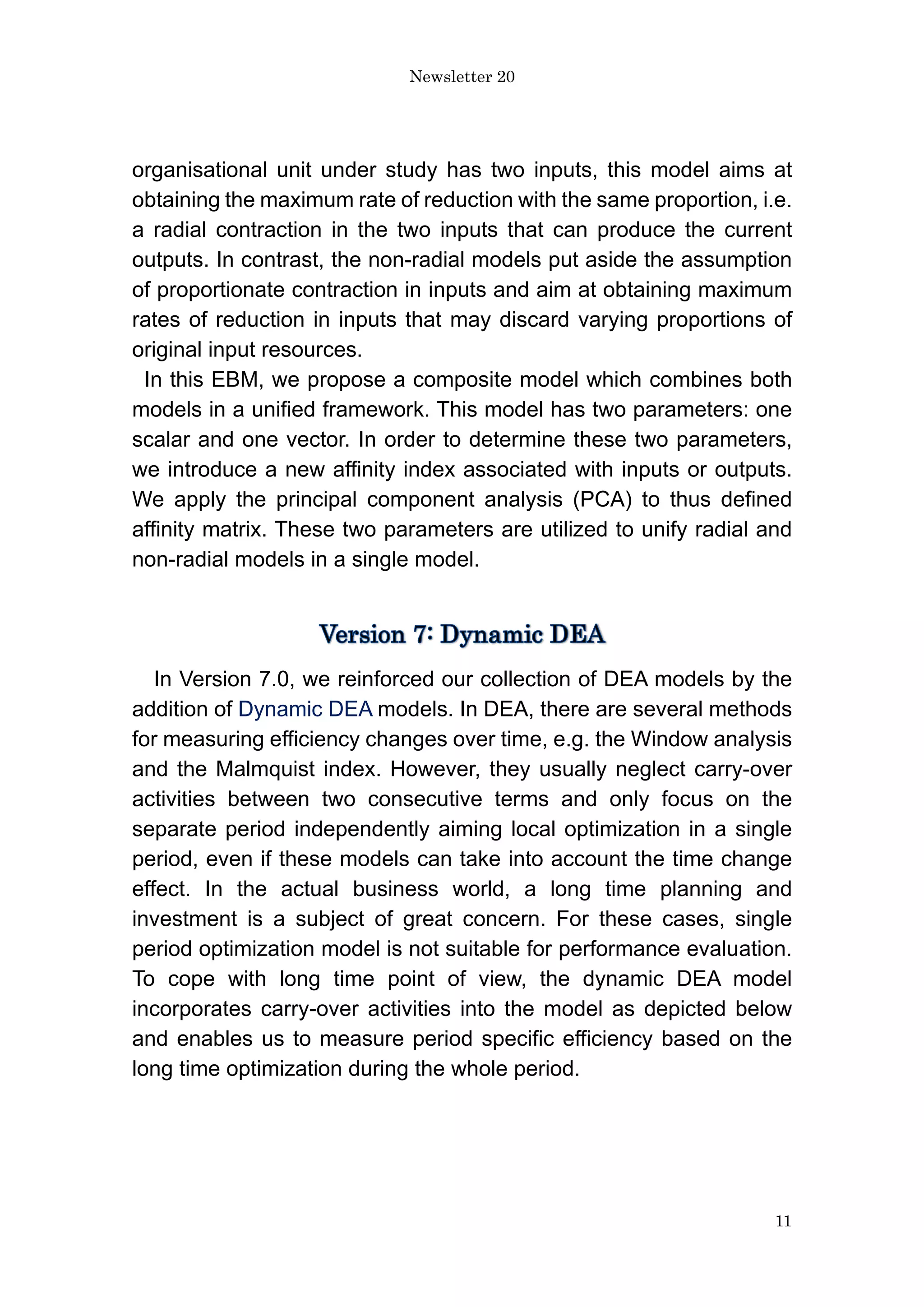
In this EBM, we propose a composite model which combines both
models in a unified framework. This model has two parameters: one
scalar and one vector. In order to determine these two parameters,
we introduce a new affinity index associated with inputs or outputs.
We apply the principal component analysis (PCA) to thus defined
affinity matrix. These two parameters are utilized to unify radial and
non-radial models in a single model.
In Version 7.0, we reinforced our collection of DEA models by the
addition of Dynamic DEA models. In DEA, there are several methods
for measuring efficiency changes over time, e.g. the Window analysis
and the Malmquist index. However, they usually neglect carry-over
activities between two consecutive terms and only focus on the
separate period independently aiming local optimization in a single
period, even if these models can take into account the time change
effect. In the actual business world, a long time planning and
investment is a subject of great concern. For these cases, single
period optimization model is not suitable for performance evaluation.
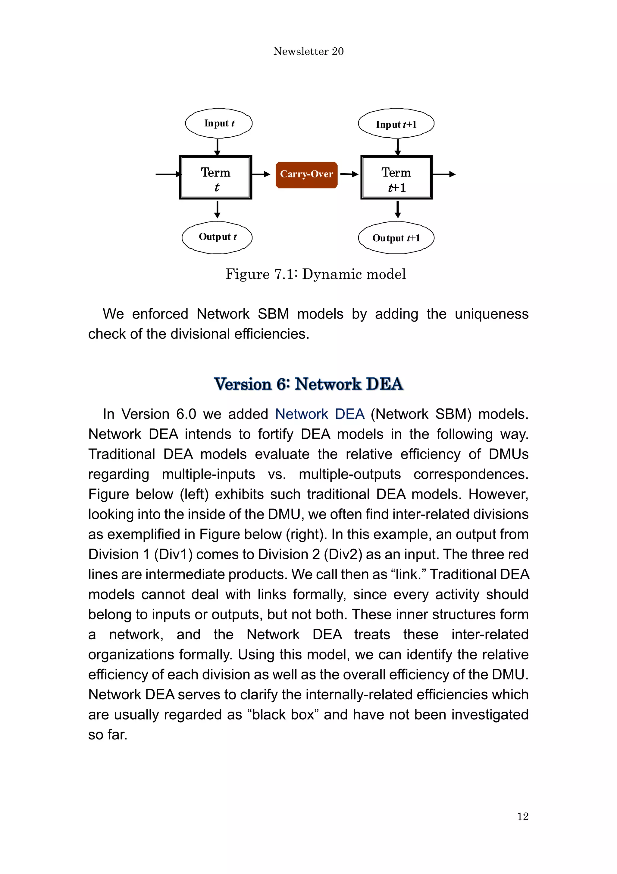
To cope with long time point of view, the dynamic DEA model
incorporates carry-over activities into the model as depicted below
and enables us to measure period specific efficiency based on the
long time optimization during the whole period.
Newsletter 20
12
Input t
Output t
Term
t
Term
t+1
Carry-Over
Output t+1
Input t+1
Figure 7.1: Dynamic model
We enforced Network SBM models by adding the uniqueness
check of the divisional efficiencies.
In Version 6.0 we added Network DEA (Network SBM) models.
Network DEA intends to fortify DEA models in the following way.
Traditional DEA models evaluate the relative efficiency of DMUs
regarding multiple-inputs vs. multiple-outputs correspondences.
Figure below (left) exhibits such traditional DEA models. However,
looking into the inside of the DMU, we often find inter-related divisions
as exemplified in Figure below (right). In this example, an output from
Division 1 (Div1) comes to Division 2 (Div2) as an input. The three red
lines are intermediate products. We call then as “link.” Traditional DEA
models cannot deal with links formally, since every activity should
belong to inputs or outputs, but not both. These inner structures form
a network, and the Network DEA treats these inter-related
organizations formally. Using this model, we can identify the relative
efficiency of each division as well as the overall efficiency of the DMU.
Network DEA serves to clarify the internally-related efficiencies which
are usually regarded as “black box” and have not been investigated
so far.
Newsletter 20
13
In Version 5.0, we added our collection of DEA models by the
Hybrid model and the Weighted SBM model, and modified the Non-
separable Outputs model in the Undesirable Outputs cluster. We also
added worksheets “Decomposition” to the SBM-family and Non-
separable Output models. This includes the decomposition of
efficiency score into inefficiency of each input/output factor.
The Hybrid model deals with radial and non-radial inputs/outputs in
a unified framework. The Weighted SBM model puts weights to slacks
in accordance with their importance to management.
In Version 4.1, we enriched our collection of DEA models by the
addition of Undesirable Outputs models. In accordance with the
global environmental conservation awareness, undesirable outputs of
production and social activities, e.g., air pollutants and hazardous
waste, have been widely recognized as societal evils. Thus,
development of technologies with less undesirable outputs is an
important subject of concern in every area of production. DEA usually
assumes that producing more outputs relative to less input resources
Input Output
Newsletter 20
14
is a criterion of efficiency. In the presence of undesirable outputs,
however, technologies with more good (desirable) outputs and less
bad (undesirable) outputs relative to less input resources should be
recognized as efficient. The Undesirable Model deals with this
problem. Please see Newsletter 5.
All DEA models can be classified into four types: (1) Radial, (2)
Non-Radial and Oriented, (3) Non-Radial and Non-Oriented and (4)
Composite of Radial and Non-radial. ‘Radial’ means that a
proportionate change of input/output values is the main concern and
hence it neglects the existence of slacks (input excesses and output
shortfalls remaining in the model) as secondary or freely disposable,
whereas ‘Non-Radial’ deals with slacks directly and does not stick to
a proportionate change of input/output. ‘Oriented’ indicates the input
or output orientation in evaluating efficiency, i.e., the main target of
evaluation is either input reduction or output expansion. For example,
input oriented models first aim to reduce input resources to the
efficient frontier as far as possible, and then to enlarge output
products as the second objective. ‘Non-Oriented’ models deal with
input reduction and output expansion at the same time.
They are classified into the four categories as displayed below.
Category Cluster or Model
Radial CCR, BCC, IRS, DRS, AR, ARG, NCN, NDSC, BND, CAT,
SYS, Bilateral, Scale Elasticity, Congestion, Window,
Malmquist-Radial, FDH, NonConvex-Radial, Resampling –
SuperRadial DD-I(O)-C(V), SuperDD-I(O)-C(V), DD-C(V),
SuperDD-C(V)
Non-Radial and Oriented SBM-Oriented, Super-efficiency-Oriented, Malmquist,
NetworkSBM(Oriented), DynamicSBM(Oriented),
DynamicNetworkSBM(Oriented), NonConvex-SBM-I(O),
Resampling-SuperSBM(Oriented), SBM_Max(Oriented)
Super-SBM_Max (Oriented), SBM_Bounded (Oriented),
NegativeData_SBM (Oriented), NegativeData_SBM_Max
(Oriented), NegativeData_Malmquist (Oriented)
Non-Radial and Non-Oriented Cost, New-Cost, Revenue, New-Revenue, Profit, New-Profit,
Ratio, SBM-NonOriented, Super-SBM-NonOriented, Malmquist-
C (V, GRS), Undesirable Outputs, Weighted SBM ,
NetworkSBM(NonOriented), DynamicSBM(NonOriented),
Bilateral, DynamicNetworkSBM(NonOriented), NonConvex-
SBM-NonOriented, Resampling-SuperSBM(NonOriented), SBM
Newsletter 20
15
Max (NonOriented)
Super-SBM_Max (NonOriented), SBM_Bounded (NonOriented)
NegativeData_SBM (NonOriented), NegativeData_SuperSBM
(NonOriented), NegativeData_Malmquist (NonOriented)
Radial and Non-Radial Hybrid, EBM
The following 56 clusters are included.
No. Cluster Model
1 CCR CCR-I, CCR-O
2 BCC BCC-I, BCC-O
3 IRS IRS-I, IRS-O
4 DRS DRS-I, DRS-O
5 GRS GRS-I, GRS-O
6 AR (assurance region) AR-I-C, AR-I-V, AR-I-GRS, AR-O-C, AR-O-V, AR-O-
GRS
7 ARG (assurance region
global)
ARG-I-C, ARG-I-V, ARG-I-GRS, ARG-O-C, ARG-O-
V, ARG-O-GRS
8 NCN (non-controllable) NCN-I-C, NCN-I-V, NCN-O-C, NCN-O-V
9 NDSC (non-discretionary) NDSC-I-C, NDSC-I-V, NDSC-I-GRS, NDSC-O-C,
NDSC-O-V, NDSC-O-GRS
10 BND (bounded variable) BND-I-C, BND-I-V, BND-I-GRS, BND-O-C, BND-O-V,
BND-O-GRS
11 CAT (categorical variable) CAT-I-C, CAT-I-V, CAT-O-C, CAT-O-V
12 SYS (different systems) SYS-I-C, SYS-I-V, SYS-O-C, SYS-O-V
13 SBM-Oriented (Slacks-based
Measure)
SBM-I-C, SBM-I-V, SBM-I-GRS, SBM-O-C, SBM-O-
V, SBM-O-GRS, SBM-AR-I-C, SBM-AR-I-V, SBM-
AR-O-C, SBM-AR-O-V
14 SBM-Non Oriented SBM-C, SBM-V, SBM-GRS, SBM-AR-C, SBM-AR-V
15 Weighted SBM WeightedSBM-C, WeightedSBM-V, WeightedSBM-I-
C,
WeightedSBM-I-V, WeightedSBM-O-C,
WeightedSBM-O-V
16 Super-SBM-Oriented Super-SBM-I-C, Super-SBM-I-V, Super-SBM-I-GRS,
Super-SBM-O-C, Super-SBM-O-V, Super-SBM-O-
GRS
17 Super-SBM-NonOriented Super-SBM-C, Super-SBM-V, Super-SBM-GRS
18 Super-Radial Super-CCR-I, Super-CCR-O, Super-BCC-I, Super-
BCC-O
19 Cost Cost-C, Cost-V, Cost-GRS
20 New-Cost New-Cost-C, New-Cost-V, New-Cost-GRS
21 Revenue Revenue-C, Revenue-V, Revenue-GRS
22 New-Revenue New-Revenue-C, New-Revenue-V, New-Revenue-GRS
23 Profit Profit-C, Profit-V, Profit-GRS
24 New-Profit New-Profit-C, New-Profit-V, New-Profit-GRS
25 Ratio (Revenue/Cost) Ratio-C, Ratio-V
26 Bilateral Bilateral-CCR-I, Bilateral-BCC-I, Bilateral-SBM-C,
Bilateral-SBM-V
27 Window Window-I-C, Window-I-V, Window-I-GRS, Window-
O-C, Window-O-V, Window-O-GRS
28 FDH FDH
29 Malmquist-NonRadial Malmquist-I-C, Malmquist-I-V, Malmquist-I-GRS,
Malmquist-O-C, Malmquist-O-V, Malmquist-O-GRS,
Malmquist-C, Malmquist-V, Malmquist-GRS
Newsletter 20
16
30 Malmquist-Radial Malmquist-Radial-I-C, Malmquist-Radial-I-V,
Malmquist-Radial-I-GRS, Malmquist-Radial-O-C,
Malmquist-Radial-O-V, Malmquist-Radial-O-GRS
31 Scale Elasticity Elasticity-I, Elasticity-O
32 Congestion Congestion
33 Undesirable outputs BadOutput-C, BadOutput-V, BadOutput-GRS,
NonSeparable-C, NonSeparable-V, NonSeparable-
GRS
34 Hybrid Hybrid-C, Hybrid-V, Hybrid-I-C, Hybrid-I-V, Hybrid-
O-C, Hybrid-O-V
35 Network DEA Oriented NetworkSBM-I(O)-C(V)
36 Network DEA Non-Oriented NetwrokSBM-C(V)
37 Dynamic DEA Oriented DynamicSBM-I(O)-C(V)
38 Dynamic DEA Non-oriented DynamicSBM-C(V)
39 EBM Oriented EBM-I(O)-C(V)
40 EBM Non-Oriented EBM-C(V)
41 DynamicNetworkSBM
Oriented
DNSBM-I-C(V), DNSBM-O-C(V)
42 DynamicNetworkSBM
NonOriented
DNSBM-C(V)
43 NonConvex-SBM NonConvex-SBM-I(O),-NonOriented
44 NonConvex-Radial NonConvex-Radial-I(O)
45 Rsampling-Triangular Resampling-(Super)SBM, Resampling-(Super)Radial
46 Resampling-Triangular-
Historical
Resampling-(Super)SBM, Resampling-(Super)Radial
47 Resampling-PastPresent Resampling-(Super)SBM, Resampling-(Super)Radial
48 Resampling-
PastPresentFuture
Resampling-(Super)SBM, Resampling-(Super)Radial
49 Directional Distance
Oriented
DD-I(O)-C(V), SuperDD-I(O)-C(V)
50 Directional Distance Non-
oriented
DD-C(V), SuperDD-C(V)
51 SBM_Max SBM_Max-I(O)-C(V), -C(V), -GRS
52 Super-SBM_Max Super-SBM_Max (Oriented), Super-SBM_Max
(NonOriented)
53 SBM_Bounded SBM_Bounded (Oriented), SBM_Bounded
(NonOriented)
54 NegativeData_SBM NegativeData_SBM-I(O)-C(V), NegativeData_SBM-
C(V), NegativeData_SuperSBM-C(V)
55 NegativeData_SBM_Max NegativeData_SBM_Max-I(O)-C(V),
NegativeData_SBM_Max-C(V)
56 NegativeData_Malmquist NegativeData_Malmquist_SBM-I(O)-C(V),
NegativeData_Malmquist_SBM-C(V)
57 Desirable Inputs GoodInpt-C, GoodInput-V
The meanings of the extensions -C, -V and –GRS are as follows.
Every DEA model assumes a returns to scale (RTS) characteristics
that is represneted by the range (L, U) of the sum of the intensity
vectorλ. The constant RTS (-C) corresponds to (L=0, U=infinity) and
Newsletter 20
17
the variable RTS (-V) to (L=1, U=1), respectively.
In the models with the extension GRS, we have to supply L and U
from keyboard, the defaults being L=0.8 and U=1.2. The increasing
RTS (IRS) corresponds to (L=1, U=infinity) and the decreasing RTS
(DRS) to (L=0, U=1), respectively. It is recommended to try several
sets of (L, U) in order to identify how the RTS chracteristics exerts an
influence on the efficiency score. In the Non-Oriented EBM models
(EBM-C and EBM-V), we must supply L and U from the keyboard, the
defaults being L=U=1.
In the Resampling models, the number of replicas must be supplied
through the keyboard.

More Related Content

Similar to Newsletter 20.pdf

IRJET- Developed Method for Optimal Solution of Transportation Problem
IRJET- Developed Method for Optimal Solution of Transportation ProblemIRJET- Developed Method for Optimal Solution of Transportation Problem
IRJET- Developed Method for Optimal Solution of Transportation Problem
IRJET Journal
 
German credit score shivaram prakash
German credit score shivaram prakashGerman credit score shivaram prakash
German credit score shivaram prakash
Shivaram Prakash
 
Chapter 5.TRANSPORTATION PROBLEM.pdf
Chapter 5.TRANSPORTATION PROBLEM.pdfChapter 5.TRANSPORTATION PROBLEM.pdf
Chapter 5.TRANSPORTATION PROBLEM.pdf
Tsegay Berhe
 
Churn Analysis in Telecom Industry
Churn Analysis in Telecom IndustryChurn Analysis in Telecom Industry
Churn Analysis in Telecom Industry
Satyam Barsaiyan
 
COST NOTES LECTURE ALL COST CURVES NUMERICALS EXAMPLES THEORY
COST NOTES LECTURE ALL COST CURVES NUMERICALS EXAMPLES THEORY COST NOTES LECTURE ALL COST CURVES NUMERICALS EXAMPLES THEORY
COST NOTES LECTURE ALL COST CURVES NUMERICALS EXAMPLES THEORY
SOURAV DAS
 
A Weighted Duality based Formulation of MIMO Systems
A Weighted Duality based Formulation of MIMO SystemsA Weighted Duality based Formulation of MIMO Systems
A Weighted Duality based Formulation of MIMO Systems
IJERA Editor
 
Can you Deep Learn the Stock Market?
Can you Deep Learn the Stock Market?Can you Deep Learn the Stock Market?
Can you Deep Learn the Stock Market?
Gaetan Lion
 
Multiple Regression
Multiple RegressionMultiple Regression
Multiple Regression
Nicholas Manurung
 
Exploring Support Vector Regression - Signals and Systems Project
Exploring Support Vector Regression - Signals and Systems ProjectExploring Support Vector Regression - Signals and Systems Project
Exploring Support Vector Regression - Signals and Systems Project
Surya Chandra
 
SupportVectorRegression
SupportVectorRegressionSupportVectorRegression
SupportVectorRegressionDaniel K
 
Sorm model for negative input s
Sorm model for negative input sSorm model for negative input s
Sorm model for negative input sGeetika Sharma
 
SOLVING A MULTI-OBJECTIVE REACTIVE POWER MARKET CLEARING MODEL USING NSGA-II
SOLVING A MULTI-OBJECTIVE REACTIVE POWER MARKET CLEARING MODEL USING NSGA-IISOLVING A MULTI-OBJECTIVE REACTIVE POWER MARKET CLEARING MODEL USING NSGA-II
SOLVING A MULTI-OBJECTIVE REACTIVE POWER MARKET CLEARING MODEL USING NSGA-II
ijait
 
Machine learning in credit risk modeling : a James white paper
Machine learning in credit risk modeling : a James white paperMachine learning in credit risk modeling : a James white paper
Machine learning in credit risk modeling : a James white paper
James by CrowdProcess
 
ASSESSMENT OF INTRICATE DG PLANNING WITH PRACTICAL LOAD MODELS BY USING PSO
ASSESSMENT OF INTRICATE DG PLANNING WITH PRACTICAL LOAD MODELS BY USING PSO ASSESSMENT OF INTRICATE DG PLANNING WITH PRACTICAL LOAD MODELS BY USING PSO
ASSESSMENT OF INTRICATE DG PLANNING WITH PRACTICAL LOAD MODELS BY USING PSO
ecij
 
11 7986 9062-1-pb
11 7986 9062-1-pb11 7986 9062-1-pb
11 7986 9062-1-pb
IAESIJEECS
 
Data envelopment analysis
Data envelopment analysisData envelopment analysis
Data envelopment analysisGlory Maker
 
Lecture6 xing
Lecture6 xingLecture6 xing
Lecture6 xing
Tianlu Wang
 
Economic Dispatch of Generated Power Using Modified Lambda-Iteration Method
Economic Dispatch of Generated Power Using Modified Lambda-Iteration MethodEconomic Dispatch of Generated Power Using Modified Lambda-Iteration Method
Economic Dispatch of Generated Power Using Modified Lambda-Iteration Method
IOSR Journals
 
Conventional and-pso-based-approaches-for-model-reduction-of-siso-discrete-sy...
Conventional and-pso-based-approaches-for-model-reduction-of-siso-discrete-sy...Conventional and-pso-based-approaches-for-model-reduction-of-siso-discrete-sy...
Conventional and-pso-based-approaches-for-model-reduction-of-siso-discrete-sy...Cemal Ardil
 

Similar to Newsletter 20.pdf (20)

IRJET- Developed Method for Optimal Solution of Transportation Problem
IRJET- Developed Method for Optimal Solution of Transportation ProblemIRJET- Developed Method for Optimal Solution of Transportation Problem
IRJET- Developed Method for Optimal Solution of Transportation Problem
 
German credit score shivaram prakash
German credit score shivaram prakashGerman credit score shivaram prakash
German credit score shivaram prakash
 
Chapter 5.TRANSPORTATION PROBLEM.pdf
Chapter 5.TRANSPORTATION PROBLEM.pdfChapter 5.TRANSPORTATION PROBLEM.pdf
Chapter 5.TRANSPORTATION PROBLEM.pdf
 
Churn Analysis in Telecom Industry
Churn Analysis in Telecom IndustryChurn Analysis in Telecom Industry
Churn Analysis in Telecom Industry
 
COST NOTES LECTURE ALL COST CURVES NUMERICALS EXAMPLES THEORY
COST NOTES LECTURE ALL COST CURVES NUMERICALS EXAMPLES THEORY COST NOTES LECTURE ALL COST CURVES NUMERICALS EXAMPLES THEORY
COST NOTES LECTURE ALL COST CURVES NUMERICALS EXAMPLES THEORY
 
A Weighted Duality based Formulation of MIMO Systems
A Weighted Duality based Formulation of MIMO SystemsA Weighted Duality based Formulation of MIMO Systems
A Weighted Duality based Formulation of MIMO Systems
 
Can you Deep Learn the Stock Market?
Can you Deep Learn the Stock Market?Can you Deep Learn the Stock Market?
Can you Deep Learn the Stock Market?
 
Multiple Regression
Multiple RegressionMultiple Regression
Multiple Regression
 
Exploring Support Vector Regression - Signals and Systems Project
Exploring Support Vector Regression - Signals and Systems ProjectExploring Support Vector Regression - Signals and Systems Project
Exploring Support Vector Regression - Signals and Systems Project
 
SupportVectorRegression
SupportVectorRegressionSupportVectorRegression
SupportVectorRegression
 
Sorm model for negative input s
Sorm model for negative input sSorm model for negative input s
Sorm model for negative input s
 
SOLVING A MULTI-OBJECTIVE REACTIVE POWER MARKET CLEARING MODEL USING NSGA-II
SOLVING A MULTI-OBJECTIVE REACTIVE POWER MARKET CLEARING MODEL USING NSGA-IISOLVING A MULTI-OBJECTIVE REACTIVE POWER MARKET CLEARING MODEL USING NSGA-II
SOLVING A MULTI-OBJECTIVE REACTIVE POWER MARKET CLEARING MODEL USING NSGA-II
 
Machine learning in credit risk modeling : a James white paper
Machine learning in credit risk modeling : a James white paperMachine learning in credit risk modeling : a James white paper
Machine learning in credit risk modeling : a James white paper
 
ASSESSMENT OF INTRICATE DG PLANNING WITH PRACTICAL LOAD MODELS BY USING PSO
ASSESSMENT OF INTRICATE DG PLANNING WITH PRACTICAL LOAD MODELS BY USING PSO ASSESSMENT OF INTRICATE DG PLANNING WITH PRACTICAL LOAD MODELS BY USING PSO
ASSESSMENT OF INTRICATE DG PLANNING WITH PRACTICAL LOAD MODELS BY USING PSO
 
11 7986 9062-1-pb
11 7986 9062-1-pb11 7986 9062-1-pb
11 7986 9062-1-pb
 
Group5
Group5Group5
Group5
 
Data envelopment analysis
Data envelopment analysisData envelopment analysis
Data envelopment analysis
 
Lecture6 xing
Lecture6 xingLecture6 xing
Lecture6 xing
 
Economic Dispatch of Generated Power Using Modified Lambda-Iteration Method
Economic Dispatch of Generated Power Using Modified Lambda-Iteration MethodEconomic Dispatch of Generated Power Using Modified Lambda-Iteration Method
Economic Dispatch of Generated Power Using Modified Lambda-Iteration Method
 
Conventional and-pso-based-approaches-for-model-reduction-of-siso-discrete-sy...
Conventional and-pso-based-approaches-for-model-reduction-of-siso-discrete-sy...Conventional and-pso-based-approaches-for-model-reduction-of-siso-discrete-sy...
Conventional and-pso-based-approaches-for-model-reduction-of-siso-discrete-sy...
 

More from Cheer Chain Enterprise Co., Ltd.

Intel® Tiber™ Developer Cloud Overview (30 min).pdf
Intel® Tiber™ Developer Cloud Overview  (30 min).pdfIntel® Tiber™ Developer Cloud Overview  (30 min).pdf
Intel® Tiber™ Developer Cloud Overview (30 min).pdf
Cheer Chain Enterprise Co., Ltd.
 
MAXQDA-24-Features-EN.pdf
MAXQDA-24-Features-EN.pdfMAXQDA-24-Features-EN.pdf
MAXQDA-24-Features-EN.pdf
Cheer Chain Enterprise Co., Ltd.
 
Paessler_Sales_Presentation_EN.pptx
Paessler_Sales_Presentation_EN.pptxPaessler_Sales_Presentation_EN.pptx
Paessler_Sales_Presentation_EN.pptx
Cheer Chain Enterprise Co., Ltd.
 
A General Method for Estimating a Linear Structural Equation System
 A General Method for Estimating a Linear Structural Equation System A General Method for Estimating a Linear Structural Equation System
A General Method for Estimating a Linear Structural Equation System
Cheer Chain Enterprise Co., Ltd.
 
Focused Analysis of #Qualitative #Interviews with #MAXQDA Step by Step - #免費 ...
Focused Analysis of #Qualitative #Interviews with #MAXQDA Step by Step - #免費 ...Focused Analysis of #Qualitative #Interviews with #MAXQDA Step by Step - #免費 ...
Focused Analysis of #Qualitative #Interviews with #MAXQDA Step by Step - #免費 ...
Cheer Chain Enterprise Co., Ltd.
 
Maxqda 2020 質性分析及混合研究理論應用軟體完整使用手冊(英文版)
Maxqda 2020 質性分析及混合研究理論應用軟體完整使用手冊(英文版)Maxqda 2020 質性分析及混合研究理論應用軟體完整使用手冊(英文版)
Maxqda 2020 質性分析及混合研究理論應用軟體完整使用手冊(英文版)
Cheer Chain Enterprise Co., Ltd.
 
#Acunetix #product #presentation
#Acunetix #product #presentation#Acunetix #product #presentation
#Acunetix #product #presentation
Cheer Chain Enterprise Co., Ltd.
 
#Riverflow2 d gpu tests 2019
#Riverflow2 d gpu tests 2019#Riverflow2 d gpu tests 2019
#Riverflow2 d gpu tests 2019
Cheer Chain Enterprise Co., Ltd.
 
Doctor web Company profile 防毒軟體公司簡介
Doctor web Company profile 防毒軟體公司簡介Doctor web Company profile 防毒軟體公司簡介
Doctor web Company profile 防毒軟體公司簡介
Cheer Chain Enterprise Co., Ltd.
 
Getting started-guide-maxqda2018 MAXQDA 2018 質性分析軟體 中英文快速入門手冊
Getting started-guide-maxqda2018 MAXQDA 2018 質性分析軟體 中英文快速入門手冊Getting started-guide-maxqda2018 MAXQDA 2018 質性分析軟體 中英文快速入門手冊
Getting started-guide-maxqda2018 MAXQDA 2018 質性分析軟體 中英文快速入門手冊
Cheer Chain Enterprise Co., Ltd.
 
NativeJ screenshot - NativeJ is a powerful Java EXE maker!
NativeJ screenshot - NativeJ is a powerful Java EXE maker!NativeJ screenshot - NativeJ is a powerful Java EXE maker!
NativeJ screenshot - NativeJ is a powerful Java EXE maker!
Cheer Chain Enterprise Co., Ltd.
 
Edraw Max Pro 使用者手冊 - All-In-One Diagram Software!!
Edraw Max Pro  使用者手冊 - All-In-One Diagram Software!!Edraw Max Pro  使用者手冊 - All-In-One Diagram Software!!
Edraw Max Pro 使用者手冊 - All-In-One Diagram Software!!
Cheer Chain Enterprise Co., Ltd.
 
Nvidia gpu-application-catalog TESLA K80 GPU應用程式型錄
Nvidia gpu-application-catalog TESLA K80 GPU應用程式型錄Nvidia gpu-application-catalog TESLA K80 GPU應用程式型錄
Nvidia gpu-application-catalog TESLA K80 GPU應用程式型錄
Cheer Chain Enterprise Co., Ltd.
 
Atlas.ti 8 質性分析軟體新功能介紹_祺荃企業有限公司
Atlas.ti 8 質性分析軟體新功能介紹_祺荃企業有限公司Atlas.ti 8 質性分析軟體新功能介紹_祺荃企業有限公司
Atlas.ti 8 質性分析軟體新功能介紹_祺荃企業有限公司
Cheer Chain Enterprise Co., Ltd.
 
Maxqda12 features -detailed feature comparison for more information about eac...
Maxqda12 features -detailed feature comparison for more information about eac...Maxqda12 features -detailed feature comparison for more information about eac...
Maxqda12 features -detailed feature comparison for more information about eac...
Cheer Chain Enterprise Co., Ltd.
 
CABRI® 3D V2 - 革命性的數學工具(中文操作手冊)
CABRI® 3D V2 - 革命性的數學工具(中文操作手冊)CABRI® 3D V2 - 革命性的數學工具(中文操作手冊)
CABRI® 3D V2 - 革命性的數學工具(中文操作手冊)
Cheer Chain Enterprise Co., Ltd.
 
MAXQDA 12 質性(定性)分析軟體中文入門指南
MAXQDA 12 質性(定性)分析軟體中文入門指南MAXQDA 12 質性(定性)分析軟體中文入門指南
MAXQDA 12 質性(定性)分析軟體中文入門指南
Cheer Chain Enterprise Co., Ltd.
 
全新 Veeam Availability Suite v9包括 Veeam Backup & Replication 和 Veeam ONE 備份解決方...
全新 Veeam Availability Suite v9包括 Veeam Backup & Replication 和 Veeam ONE 備份解決方...全新 Veeam Availability Suite v9包括 Veeam Backup & Replication 和 Veeam ONE 備份解決方...
全新 Veeam Availability Suite v9包括 Veeam Backup & Replication 和 Veeam ONE 備份解決方...
Cheer Chain Enterprise Co., Ltd.
 
AVG 2016 business edition customer deck - 屢獲殊榮的防毒軟體保護您的企業免於最新的威脅與病毒
AVG 2016 business edition customer deck - 屢獲殊榮的防毒軟體保護您的企業免於最新的威脅與病毒AVG 2016 business edition customer deck - 屢獲殊榮的防毒軟體保護您的企業免於最新的威脅與病毒
AVG 2016 business edition customer deck - 屢獲殊榮的防毒軟體保護您的企業免於最新的威脅與病毒
Cheer Chain Enterprise Co., Ltd.
 
德國 combit List & label 21 報表設計工具軟體新功能介紹
德國 combit List & label 21 報表設計工具軟體新功能介紹德國 combit List & label 21 報表設計工具軟體新功能介紹
德國 combit List & label 21 報表設計工具軟體新功能介紹
Cheer Chain Enterprise Co., Ltd.
 

More from Cheer Chain Enterprise Co., Ltd. (20)

Intel® Tiber™ Developer Cloud Overview (30 min).pdf
Intel® Tiber™ Developer Cloud Overview  (30 min).pdfIntel® Tiber™ Developer Cloud Overview  (30 min).pdf
Intel® Tiber™ Developer Cloud Overview (30 min).pdf
 
MAXQDA-24-Features-EN.pdf
MAXQDA-24-Features-EN.pdfMAXQDA-24-Features-EN.pdf
MAXQDA-24-Features-EN.pdf
 
Paessler_Sales_Presentation_EN.pptx
Paessler_Sales_Presentation_EN.pptxPaessler_Sales_Presentation_EN.pptx
Paessler_Sales_Presentation_EN.pptx
 
A General Method for Estimating a Linear Structural Equation System
 A General Method for Estimating a Linear Structural Equation System A General Method for Estimating a Linear Structural Equation System
A General Method for Estimating a Linear Structural Equation System
 
Focused Analysis of #Qualitative #Interviews with #MAXQDA Step by Step - #免費 ...
Focused Analysis of #Qualitative #Interviews with #MAXQDA Step by Step - #免費 ...Focused Analysis of #Qualitative #Interviews with #MAXQDA Step by Step - #免費 ...
Focused Analysis of #Qualitative #Interviews with #MAXQDA Step by Step - #免費 ...
 
Maxqda 2020 質性分析及混合研究理論應用軟體完整使用手冊(英文版)
Maxqda 2020 質性分析及混合研究理論應用軟體完整使用手冊(英文版)Maxqda 2020 質性分析及混合研究理論應用軟體完整使用手冊(英文版)
Maxqda 2020 質性分析及混合研究理論應用軟體完整使用手冊(英文版)
 
#Acunetix #product #presentation
#Acunetix #product #presentation#Acunetix #product #presentation
#Acunetix #product #presentation
 
#Riverflow2 d gpu tests 2019
#Riverflow2 d gpu tests 2019#Riverflow2 d gpu tests 2019
#Riverflow2 d gpu tests 2019
 
Doctor web Company profile 防毒軟體公司簡介
Doctor web Company profile 防毒軟體公司簡介Doctor web Company profile 防毒軟體公司簡介
Doctor web Company profile 防毒軟體公司簡介
 
Getting started-guide-maxqda2018 MAXQDA 2018 質性分析軟體 中英文快速入門手冊
Getting started-guide-maxqda2018 MAXQDA 2018 質性分析軟體 中英文快速入門手冊Getting started-guide-maxqda2018 MAXQDA 2018 質性分析軟體 中英文快速入門手冊
Getting started-guide-maxqda2018 MAXQDA 2018 質性分析軟體 中英文快速入門手冊
 
NativeJ screenshot - NativeJ is a powerful Java EXE maker!
NativeJ screenshot - NativeJ is a powerful Java EXE maker!NativeJ screenshot - NativeJ is a powerful Java EXE maker!
NativeJ screenshot - NativeJ is a powerful Java EXE maker!
 
Edraw Max Pro 使用者手冊 - All-In-One Diagram Software!!
Edraw Max Pro  使用者手冊 - All-In-One Diagram Software!!Edraw Max Pro  使用者手冊 - All-In-One Diagram Software!!
Edraw Max Pro 使用者手冊 - All-In-One Diagram Software!!
 
Nvidia gpu-application-catalog TESLA K80 GPU應用程式型錄
Nvidia gpu-application-catalog TESLA K80 GPU應用程式型錄Nvidia gpu-application-catalog TESLA K80 GPU應用程式型錄
Nvidia gpu-application-catalog TESLA K80 GPU應用程式型錄
 
Atlas.ti 8 質性分析軟體新功能介紹_祺荃企業有限公司
Atlas.ti 8 質性分析軟體新功能介紹_祺荃企業有限公司Atlas.ti 8 質性分析軟體新功能介紹_祺荃企業有限公司
Atlas.ti 8 質性分析軟體新功能介紹_祺荃企業有限公司
 
Maxqda12 features -detailed feature comparison for more information about eac...
Maxqda12 features -detailed feature comparison for more information about eac...Maxqda12 features -detailed feature comparison for more information about eac...
Maxqda12 features -detailed feature comparison for more information about eac...
 
CABRI® 3D V2 - 革命性的數學工具(中文操作手冊)
CABRI® 3D V2 - 革命性的數學工具(中文操作手冊)CABRI® 3D V2 - 革命性的數學工具(中文操作手冊)
CABRI® 3D V2 - 革命性的數學工具(中文操作手冊)
 
MAXQDA 12 質性(定性)分析軟體中文入門指南
MAXQDA 12 質性(定性)分析軟體中文入門指南MAXQDA 12 質性(定性)分析軟體中文入門指南
MAXQDA 12 質性(定性)分析軟體中文入門指南
 
全新 Veeam Availability Suite v9包括 Veeam Backup & Replication 和 Veeam ONE 備份解決方...
全新 Veeam Availability Suite v9包括 Veeam Backup & Replication 和 Veeam ONE 備份解決方...全新 Veeam Availability Suite v9包括 Veeam Backup & Replication 和 Veeam ONE 備份解決方...
全新 Veeam Availability Suite v9包括 Veeam Backup & Replication 和 Veeam ONE 備份解決方...
 
AVG 2016 business edition customer deck - 屢獲殊榮的防毒軟體保護您的企業免於最新的威脅與病毒
AVG 2016 business edition customer deck - 屢獲殊榮的防毒軟體保護您的企業免於最新的威脅與病毒AVG 2016 business edition customer deck - 屢獲殊榮的防毒軟體保護您的企業免於最新的威脅與病毒
AVG 2016 business edition customer deck - 屢獲殊榮的防毒軟體保護您的企業免於最新的威脅與病毒
 
德國 combit List & label 21 報表設計工具軟體新功能介紹
德國 combit List & label 21 報表設計工具軟體新功能介紹德國 combit List & label 21 報表設計工具軟體新功能介紹
德國 combit List & label 21 報表設計工具軟體新功能介紹
 

Recently uploaded

A Comprehensive Look at Generative AI in Retail App Testing.pdf
A Comprehensive Look at Generative AI in Retail App Testing.pdfA Comprehensive Look at Generative AI in Retail App Testing.pdf
A Comprehensive Look at Generative AI in Retail App Testing.pdf
kalichargn70th171
 
Field Employee Tracking System| MiTrack App| Best Employee Tracking Solution|...
Field Employee Tracking System| MiTrack App| Best Employee Tracking Solution|...Field Employee Tracking System| MiTrack App| Best Employee Tracking Solution|...
Field Employee Tracking System| MiTrack App| Best Employee Tracking Solution|...
informapgpstrackings
 
A Sighting of filterA in Typelevel Rite of Passage
A Sighting of filterA in Typelevel Rite of PassageA Sighting of filterA in Typelevel Rite of Passage
A Sighting of filterA in Typelevel Rite of Passage
Philip Schwarz
 
Climate Science Flows: Enabling Petabyte-Scale Climate Analysis with the Eart...
Climate Science Flows: Enabling Petabyte-Scale Climate Analysis with the Eart...Climate Science Flows: Enabling Petabyte-Scale Climate Analysis with the Eart...
Climate Science Flows: Enabling Petabyte-Scale Climate Analysis with the Eart...
Globus
 
Graphic Design Crash Course for beginners
Graphic Design Crash Course for beginnersGraphic Design Crash Course for beginners
Graphic Design Crash Course for beginners
e20449
 
Cracking the code review at SpringIO 2024
Cracking the code review at SpringIO 2024Cracking the code review at SpringIO 2024
Cracking the code review at SpringIO 2024
Paco van Beckhoven
 
Large Language Models and the End of Programming
Large Language Models and the End of ProgrammingLarge Language Models and the End of Programming
Large Language Models and the End of Programming
Matt Welsh
 
Lecture 1 Introduction to games development
Lecture 1 Introduction to games developmentLecture 1 Introduction to games development
Lecture 1 Introduction to games development
abdulrafaychaudhry
 
Navigating the Metaverse: A Journey into Virtual Evolution"
Navigating the Metaverse: A Journey into Virtual Evolution"Navigating the Metaverse: A Journey into Virtual Evolution"
Navigating the Metaverse: A Journey into Virtual Evolution"
Donna Lenk
 
Into the Box 2024 - Keynote Day 2 Slides.pdf
Into the Box 2024 - Keynote Day 2 Slides.pdfInto the Box 2024 - Keynote Day 2 Slides.pdf
Into the Box 2024 - Keynote Day 2 Slides.pdf
Ortus Solutions, Corp
 
Prosigns: Transforming Business with Tailored Technology Solutions
Prosigns: Transforming Business with Tailored Technology SolutionsProsigns: Transforming Business with Tailored Technology Solutions
Prosigns: Transforming Business with Tailored Technology Solutions
Prosigns
 
AI Pilot Review: The World’s First Virtual Assistant Marketing Suite
AI Pilot Review: The World’s First Virtual Assistant Marketing SuiteAI Pilot Review: The World’s First Virtual Assistant Marketing Suite
AI Pilot Review: The World’s First Virtual Assistant Marketing Suite
Google
 
Orion Context Broker introduction 20240604
Orion Context Broker introduction 20240604Orion Context Broker introduction 20240604
Orion Context Broker introduction 20240604
Fermin Galan
 
Accelerate Enterprise Software Engineering with Platformless
Accelerate Enterprise Software Engineering with PlatformlessAccelerate Enterprise Software Engineering with Platformless
Accelerate Enterprise Software Engineering with Platformless
WSO2
 
Quarkus Hidden and Forbidden Extensions
Quarkus Hidden and Forbidden ExtensionsQuarkus Hidden and Forbidden Extensions
Quarkus Hidden and Forbidden Extensions
Max Andersen
 
TROUBLESHOOTING 9 TYPES OF OUTOFMEMORYERROR
TROUBLESHOOTING 9 TYPES OF OUTOFMEMORYERRORTROUBLESHOOTING 9 TYPES OF OUTOFMEMORYERROR
TROUBLESHOOTING 9 TYPES OF OUTOFMEMORYERROR
Tier1 app
 
How Recreation Management Software Can Streamline Your Operations.pptx
How Recreation Management Software Can Streamline Your Operations.pptxHow Recreation Management Software Can Streamline Your Operations.pptx
How Recreation Management Software Can Streamline Your Operations.pptx
wottaspaceseo
 
Innovating Inference - Remote Triggering of Large Language Models on HPC Clus...
Innovating Inference - Remote Triggering of Large Language Models on HPC Clus...Innovating Inference - Remote Triggering of Large Language Models on HPC Clus...
Innovating Inference - Remote Triggering of Large Language Models on HPC Clus...
Globus
 
Globus Connect Server Deep Dive - GlobusWorld 2024
Globus Connect Server Deep Dive - GlobusWorld 2024Globus Connect Server Deep Dive - GlobusWorld 2024
Globus Connect Server Deep Dive - GlobusWorld 2024
Globus
 
Custom Healthcare Software for Managing Chronic Conditions and Remote Patient...
Custom Healthcare Software for Managing Chronic Conditions and Remote Patient...Custom Healthcare Software for Managing Chronic Conditions and Remote Patient...
Custom Healthcare Software for Managing Chronic Conditions and Remote Patient...
Mind IT Systems
 

Recently uploaded (20)

A Comprehensive Look at Generative AI in Retail App Testing.pdf
A Comprehensive Look at Generative AI in Retail App Testing.pdfA Comprehensive Look at Generative AI in Retail App Testing.pdf
A Comprehensive Look at Generative AI in Retail App Testing.pdf
 
Field Employee Tracking System| MiTrack App| Best Employee Tracking Solution|...
Field Employee Tracking System| MiTrack App| Best Employee Tracking Solution|...Field Employee Tracking System| MiTrack App| Best Employee Tracking Solution|...
Field Employee Tracking System| MiTrack App| Best Employee Tracking Solution|...
 
A Sighting of filterA in Typelevel Rite of Passage
A Sighting of filterA in Typelevel Rite of PassageA Sighting of filterA in Typelevel Rite of Passage
A Sighting of filterA in Typelevel Rite of Passage
 
Climate Science Flows: Enabling Petabyte-Scale Climate Analysis with the Eart...
Climate Science Flows: Enabling Petabyte-Scale Climate Analysis with the Eart...Climate Science Flows: Enabling Petabyte-Scale Climate Analysis with the Eart...
Climate Science Flows: Enabling Petabyte-Scale Climate Analysis with the Eart...
 
Graphic Design Crash Course for beginners
Graphic Design Crash Course for beginnersGraphic Design Crash Course for beginners
Graphic Design Crash Course for beginners
 
Cracking the code review at SpringIO 2024
Cracking the code review at SpringIO 2024Cracking the code review at SpringIO 2024
Cracking the code review at SpringIO 2024
 
Large Language Models and the End of Programming
Large Language Models and the End of ProgrammingLarge Language Models and the End of Programming
Large Language Models and the End of Programming
 
Lecture 1 Introduction to games development
Lecture 1 Introduction to games developmentLecture 1 Introduction to games development
Lecture 1 Introduction to games development
 
Navigating the Metaverse: A Journey into Virtual Evolution"
Navigating the Metaverse: A Journey into Virtual Evolution"Navigating the Metaverse: A Journey into Virtual Evolution"
Navigating the Metaverse: A Journey into Virtual Evolution"
 
Into the Box 2024 - Keynote Day 2 Slides.pdf
Into the Box 2024 - Keynote Day 2 Slides.pdfInto the Box 2024 - Keynote Day 2 Slides.pdf
Into the Box 2024 - Keynote Day 2 Slides.pdf
 
Prosigns: Transforming Business with Tailored Technology Solutions
Prosigns: Transforming Business with Tailored Technology SolutionsProsigns: Transforming Business with Tailored Technology Solutions
Prosigns: Transforming Business with Tailored Technology Solutions
 
AI Pilot Review: The World’s First Virtual Assistant Marketing Suite
AI Pilot Review: The World’s First Virtual Assistant Marketing SuiteAI Pilot Review: The World’s First Virtual Assistant Marketing Suite
AI Pilot Review: The World’s First Virtual Assistant Marketing Suite
 
Orion Context Broker introduction 20240604
Orion Context Broker introduction 20240604Orion Context Broker introduction 20240604
Orion Context Broker introduction 20240604
 
Accelerate Enterprise Software Engineering with Platformless
Accelerate Enterprise Software Engineering with PlatformlessAccelerate Enterprise Software Engineering with Platformless
Accelerate Enterprise Software Engineering with Platformless
 
Quarkus Hidden and Forbidden Extensions
Quarkus Hidden and Forbidden ExtensionsQuarkus Hidden and Forbidden Extensions
Quarkus Hidden and Forbidden Extensions
 
TROUBLESHOOTING 9 TYPES OF OUTOFMEMORYERROR
TROUBLESHOOTING 9 TYPES OF OUTOFMEMORYERRORTROUBLESHOOTING 9 TYPES OF OUTOFMEMORYERROR
TROUBLESHOOTING 9 TYPES OF OUTOFMEMORYERROR
 
How Recreation Management Software Can Streamline Your Operations.pptx
How Recreation Management Software Can Streamline Your Operations.pptxHow Recreation Management Software Can Streamline Your Operations.pptx
How Recreation Management Software Can Streamline Your Operations.pptx
 
Innovating Inference - Remote Triggering of Large Language Models on HPC Clus...
Innovating Inference - Remote Triggering of Large Language Models on HPC Clus...Innovating Inference - Remote Triggering of Large Language Models on HPC Clus...
Innovating Inference - Remote Triggering of Large Language Models on HPC Clus...
 
Globus Connect Server Deep Dive - GlobusWorld 2024
Globus Connect Server Deep Dive - GlobusWorld 2024Globus Connect Server Deep Dive - GlobusWorld 2024
Globus Connect Server Deep Dive - GlobusWorld 2024
 
Custom Healthcare Software for Managing Chronic Conditions and Remote Patient...
Custom Healthcare Software for Managing Chronic Conditions and Remote Patient...Custom Healthcare Software for Managing Chronic Conditions and Remote Patient...
Custom Healthcare Software for Managing Chronic Conditions and Remote Patient...
 

Newsletter 20.pdf

  • 1. Newsletter 20 1 : How can we deal with big data set comprised of several thousand DMUs? : You can divide them into several groups consisting of a few hundred DMUs and solve each group for finding efficient DMUs in the group. Then, merge the efficient DMUs into one set. Solve the set and find the final efficient DMUs. Using the finalist, re-evaluate each group. Version 16.0: Desirable Inputs Model Generally speaking, in DEA, inputs (I) indicate input resources and the smaller the better, while outputs (O) correspond to productions induced by inputs (I), which are the larger the better. Among outputs, there exist undesirable outputs (OBad) incidental to outputs, e.g. CO2, which are the smaller the better. In this version, we propose a new input style, called Desirable inputs (IGood), which are the larger the better. We show four potential examples of (IGood). (a)In accordance with the increasing concern on environmental pollution, spread of Electric cars is worldwide required. We compare the energy consumption issue of countries. We consider “Number of Electric Cars” as a Good Input (IGood). Other IO items are (I) Total consumption of Energy, (O) GDP and (OBad) Pollutants (e.g. CO2). DMUs are Country 1 to Country N. (b)We consider the case that there are many new projects in a company and the manager wishes to evaluate the efficiency of projects. For this purpose, a certain number of evaluators is assigned to each project and they report Cost (Input), Return DEA-Solver-Pro Newsletter No. 20 (Jan 7, 2022)
  • 2. Newsletter 20 2 (Output), Risk (Undesirable Output) for the assigned project. In this case, we consider the number of evaluators is a Desirable input (IGood) and the larger the better. (c)We point to “Women’s Rights Movements” in a country where women’s right is not fully guaranteed. In such a country, suppose local governments where men and women are serving as officers. They are inputs to office, while women are (IGood) and men are (I). As outputs, we assume (O) Service and (OBad) Claims. (d)Suppose that, inspired by COVID-19, many medical enterprises are eager to develop vaccine. In this case, (IGood) Number of test takers, (I) Cost, (O) Recovery, (OBad) Failure. As DMUs, we assume potential Vaccine1 to Vaccine N. We reasoned that such situations occur in many fields of enterprise. We formulate this situation in the framework of SBM. In Version 15.1, we added the CRS (constant returns-to-scale) version to NegativeData_SBM models. Furthermore, as for Malmquist models, we added the cumulative and the adjusted Malmquist indices. In DEA, we often encounter negative data, e.g. financial data. In response to many requests, in this Version 15.0, we updated SBM models to cope with negative data. Three clusters are added under the Variable Returns-to-Scale (VRS) model. They are (1) NegativeData_SBM, (2) NegativeData_SBM_Max and (3) NegativeData_Malmquist. Now, we can deal with positive and negative data in a single model. The efficiency scores are units invariant and translation invariant.
  • 3. Newsletter 20 3 In Version 14.0, we introduced SBM_Bounded models as an extension of the SBM_Max models. In real world applications, there are cases where input-reduction and/or output expansion are restricted by some external constraints. For example, suppose that expansion of inpatient visits, as an output of hospitals, is bounded by 3% of the current value due to physical environments. Input reduction bound and output expansion bound differ for every input and every output. The SBM_Bounded models handle these cases as the constraints to slacks which are obtained by SBM_Max models. Hence, the projection of inefficient DMUs thus obtained indicates more practical and useful improvement (Kaizen) plan. In Figure 14.0, we illustrate the model in the input side projection. DMUs A, B, C and D are on the efficient frontier while P and S are inefficient. P will be projected to R by the SBM_Max model, whereas the bounded area forces it to stop at Q. The bounded area is determined by Input 1 reduction rate and Input 2 reduction rate which are assumed to be common to all DMUs. DMU S is projected to T inside its bounded area and on the efficient frontier. Input 1 Input 2 A B C D ●P ● Q ●S T ● R 0
  • 4. Newsletter 20 4 Figure 14.0: SBM_Bounded model In Version 14.0, we have revised the SBM_Max models. In Version 13.2, we added Super-Efficiency score to the SBM_Max model. In Version 13.0, we replaced SBM_Variation models in the earlier version by SBM_Max models. The SBM models usually report the worst efficiency scores for inefficient DMUs. This means that the projected point is the farthest one on the associated efficient frontier. In contrast, SBM_Max models look for the nearest point on the associated efficient frontier. Hence, the efficiency score is, in a sense, maximized as contrasted to the ordinary SBM (Min) models. This indicates that we can attain an efficient status with less input reductions and less output expansions than the ordinary SBM (Min) models. The relationship among SBM-Min, SBM-Max and CCR models can be depicted by the figure below. The new SBM_Max models attain more accurate nearest point on the efficient frontiers than the SBM_Variation in the previous version, whereas the computational time increases depending on the number of efficient DMUs. We can say that the projection by SBM_Max model represents a practical “KAIZEN” (Improvement) by DEA. This model includes input-, output- and non-oriented versions under the constant and variable returns-to-scale assumptions.
  • 5. Newsletter 20 5 Figure 13.1: SBM-Min, CCR and SBM-Max In Version 12.0, we introduced Directional Distance (Function) Model that computes the efficiency of DMUs along the given direction. We offer two types of efficiency, i.e., ordinary and super efficiency. The Directional Distance model (DD model) has three variations: (1) Input- (2) Output- and (3) Non-oriented. Each variation has two returns-to-scale (RTS): (a) CRS (Constant RTS) and (b) VRS (Variable RTS). The DD model deals with two kinds of input and three kinds of output as follows. (a)Directional (Ordinary) inputs (I) The heading of this class is (I) and its value is denoted by ( ) ( 1, , ; 1, , ) I ij x i I j n = =   where 1, , i I =  corresponds to input and 1, , j n =  indicates DMU. The component of directional vector is defined as ( ) ( ) I I ij ij d x = . Input 1 Input 2 O
  • 6. Newsletter 20 6 (b)Non-directional inputs (IN) The heading of this class is (IN) and denoted by ( ) ( 1, , ; 1, , ) IN ij x i IN j n = =   where IN is the number of (IN) inputs. The component of directional vector is defined as ( ) 0 IN ij d = . This class has no directional effect on the efficiency score, but associates with it through the intensity vector. This class is the secondary input and can be empty. (c)Directional (Good) output (O) The heading of this class is (O) and denoted by ( ) ( 1, ,O; 1, , ) O ij y i j n = =   where O is the number of good outputs. The component of directional vector is defined as ( ) ( ) O O ij ij d y = . (d)Non-directional outputs (ON) The heading of this class is (ON) and denoted by ( ) ( 1, ,ON; 1, , ) ON ij y i j n = =   where ON is the number of non-directional outputs. The component of directional vector is defined as ( ) 0 ON ij d = . This class has no directional effect on the efficiency score, but associates with it through the intensity vector. This class is the secondary output and can be empty. (e)Undesirable outputs (OBad) The heading of this class is (OBad) and denoted by ( ) ( 1, ,OBad; 1, , ) OBad ij y i j n = =   where OBad is the number of undesirable outputs. The component of directional vector is defined as ( ) ( ) OBad OBad ij ij d y = . This class can be empty. In Version 11.0, we introduced a new model called “Resampling in DEA”. This model deals with data variations and gives confidence
  • 7. Newsletter 20 7 intervals of DEA scores. Input/output values are subject to change for several reasons, e.g., measurement errors, hysteretic factors, arbitrariness and so on. Furthermore, these variations differ in their input/output items and their decision-making units (DMU). Hence, DEA efficiency scores need to be examined by considering these factors. Resampling based on these variations is necessary for gauging the confidence interval of DEA scores. We propose four resampling models. The first one assumes downside and upside measurement error rates for each input/output, which are common to all DMUs. We resample data following the triangular distribution that the downside and upside errors indicate around the observed data. The second model evaluates the downside and upside error rates from historical data. The third model utilizes historical data, e.g., past- present, for estimating data variations, imposing chronological order weights which are supplied by Lucas series (a variant of Fibonacci series). This model provides different downside and upside error rates for each DMU. The last one deals with future prospects. This model aims at forecasting the future efficiency score and its confidence interval for each DMU. Table 11.1 exhibits a sample of forecast DEA scores and their confidence intervals, while Figure 11.1 shows 95% confidence interval of forecast scores. Table 11.1: Forecast DEA score and confidence interval DMU Forecast 97.50% 90% 80% 75% 50% 25% 20% 10% 2.50% H1 0.946 1.122 1.092 1.062 1.036 0.925 0.880 0.870 0.849 0.818 H2 1.043 1.128 1.098 1.079 1.073 1.049 0.906 0.883 0.845 0.815 H3 0.708 0.743 0.722 0.709 0.704 0.683 0.662 0.657 0.645 0.625 H4 0.809 0.828 0.809 0.796 0.792 0.769 0.747 0.742 0.728 0.708 H5 0.719 0.748 0.727 0.714 0.709 0.689 0.668 0.663 0.651 0.633 H6 1.067 1.185 1.146 1.124 1.115 1.084 1.055 1.049 1.033 0.993 H7 0.900 0.918 0.894 0.879 0.874 0.849 0.826 0.820 0.805 0.782 H8 0.795 0.877 0.835 0.809 0.798 0.762 0.730 0.722 0.705 0.680 H9 0.689 0.736 0.707 0.689 0.681 0.655 0.630 0.623 0.606 0.582 H10 0.801 1.065 0.981 0.914 0.891 0.791 0.748 0.740 0.720 0.689 H11 0.866 1.010 0.947 0.914 0.902 0.861 0.826 0.819 0.798 0.771 H12 1.013 1.014 0.992 0.961 0.951 0.911 0.878 0.870 0.850 0.822
  • 8. Newsletter 20 8 Figure 11.1: Forecast DEA score and 95% confidence interval In Version 10.0, we introduced the “Non-convex DEA” model. In DEA, we are often puzzled by the large difference between the constant-returns-scale (CRS) and variable returns-to-scale (VRS) scores, and by the convexity production set syndrome in spite of the S-shaped curve often observed in many real data sets. See Figure 10.1. In this model, we propose a solution to these problems. 0.000 0.200 0.400 0.600 0.800 1.000 1.200 1.400 H1 H2 H3 H4 H5 H6 H7 H8 H9 H10 H11 H12 97.50% DEA 2.50% 0 1 2 3 4 5 6 7 8 0 1 2 3 4 5 6 7 8 9 10 11 y x
  • 9. Newsletter 20 9 Figure 10.1: S-shaped data In Version 9.0, we introduced a model called “DNSBM” (dynamic SBM with network structure). We have already introduced the network SBM (NSBM) and the dynamic SBM (DSBM) models separately. Hence, this model is a composite of these two models. Vertically, we deal with multiple divisions connected by links of network structure within each period and, horizontally, we combine the network structure by means of carry-over activities between two succeeding periods. See Figure 9.1 below. This model can evaluate (1) the overall efficiency over the observed entire period, (2) dynamic change of period (term) efficiency (3) dynamic change of divisional efficiency and (4) divisional Malmquist index. The model can be implemented in input-, output- or non-(both) oriented forms under the CRS or VRS assumptions on the production possibility set. We can impose the initial condition on the carry-overs. We can formally deal with bad carry-overs, such as nonperforming loans and dead stock, in this model. We modified the data formats of Dynamic SBM (DSBM) and Network SBM (NSBM) so that they are compatible with DNSBM model. Please see User’s Guide Version 10.0.
  • 10. Newsletter 20 10 Figure 9.1: Dynamic model with network structure In Version 8.0 we introduced a model called “EBM” (epsilon-based measure of efficiency) for measuring technical efficiency. DEA is a data driven tool for measuring efficiency of decision making units (DMU) and shows a sharp contrast to so-called “parametric methods” such as stochastic frontier analysis (SFA). The latter methods assume specific production function forms to be identified. This assumption is not so reasonable in several instances and aspects. Since DEA can deal with multiple inputs vs. multiple outputs relations in a single framework, it is becoming a method of choice for efficiency evaluation. However, DEA has several shortcomings to be explored further. In DEA, we have two measures of technical efficiency with different characteristics: radial and non-radial. Historically, the radial measure, represented by the CCR model was the first DEA model, whereas the non-radial model, represented by the SBM model was a latecomer. For instance, in the input-oriented case, the CCR deals mainly with proportionate reduction of input resources. In other words, if the Carry- Over Carry- Over Carry- Over Output Output 2 Output 3 Division 2 Division 3 Division 1 Link 2→3 Link 1→2 Input 2 Division 2 Division 3 Division 1 Input 3 Input 1 Output 1 Output 2 Output 3 Link 2→3 Link 1→2 Input 2 Input 3 Period t Input 1 Period t+1
  • 11. Newsletter 20 11 organisational unit under study has two inputs, this model aims at obtaining the maximum rate of reduction with the same proportion, i.e. a radial contraction in the two inputs that can produce the current outputs. In contrast, the non-radial models put aside the assumption of proportionate contraction in inputs and aim at obtaining maximum rates of reduction in inputs that may discard varying proportions of original input resources. In this EBM, we propose a composite model which combines both models in a unified framework. This model has two parameters: one scalar and one vector. In order to determine these two parameters, we introduce a new affinity index associated with inputs or outputs. We apply the principal component analysis (PCA) to thus defined affinity matrix. These two parameters are utilized to unify radial and non-radial models in a single model. In Version 7.0, we reinforced our collection of DEA models by the addition of Dynamic DEA models. In DEA, there are several methods for measuring efficiency changes over time, e.g. the Window analysis and the Malmquist index. However, they usually neglect carry-over activities between two consecutive terms and only focus on the separate period independently aiming local optimization in a single period, even if these models can take into account the time change effect. In the actual business world, a long time planning and investment is a subject of great concern. For these cases, single period optimization model is not suitable for performance evaluation. To cope with long time point of view, the dynamic DEA model incorporates carry-over activities into the model as depicted below and enables us to measure period specific efficiency based on the long time optimization during the whole period.
  • 12. Newsletter 20 12 Input t Output t Term t Term t+1 Carry-Over Output t+1 Input t+1 Figure 7.1: Dynamic model We enforced Network SBM models by adding the uniqueness check of the divisional efficiencies. In Version 6.0 we added Network DEA (Network SBM) models. Network DEA intends to fortify DEA models in the following way. Traditional DEA models evaluate the relative efficiency of DMUs regarding multiple-inputs vs. multiple-outputs correspondences. Figure below (left) exhibits such traditional DEA models. However, looking into the inside of the DMU, we often find inter-related divisions as exemplified in Figure below (right). In this example, an output from Division 1 (Div1) comes to Division 2 (Div2) as an input. The three red lines are intermediate products. We call then as “link.” Traditional DEA models cannot deal with links formally, since every activity should belong to inputs or outputs, but not both. These inner structures form a network, and the Network DEA treats these inter-related organizations formally. Using this model, we can identify the relative efficiency of each division as well as the overall efficiency of the DMU. Network DEA serves to clarify the internally-related efficiencies which are usually regarded as “black box” and have not been investigated so far.
  • 13. Newsletter 20 13 In Version 5.0, we added our collection of DEA models by the Hybrid model and the Weighted SBM model, and modified the Non- separable Outputs model in the Undesirable Outputs cluster. We also added worksheets “Decomposition” to the SBM-family and Non- separable Output models. This includes the decomposition of efficiency score into inefficiency of each input/output factor. The Hybrid model deals with radial and non-radial inputs/outputs in a unified framework. The Weighted SBM model puts weights to slacks in accordance with their importance to management. In Version 4.1, we enriched our collection of DEA models by the addition of Undesirable Outputs models. In accordance with the global environmental conservation awareness, undesirable outputs of production and social activities, e.g., air pollutants and hazardous waste, have been widely recognized as societal evils. Thus, development of technologies with less undesirable outputs is an important subject of concern in every area of production. DEA usually assumes that producing more outputs relative to less input resources Input Output
  • 14. Newsletter 20 14 is a criterion of efficiency. In the presence of undesirable outputs, however, technologies with more good (desirable) outputs and less bad (undesirable) outputs relative to less input resources should be recognized as efficient. The Undesirable Model deals with this problem. Please see Newsletter 5. All DEA models can be classified into four types: (1) Radial, (2) Non-Radial and Oriented, (3) Non-Radial and Non-Oriented and (4) Composite of Radial and Non-radial. ‘Radial’ means that a proportionate change of input/output values is the main concern and hence it neglects the existence of slacks (input excesses and output shortfalls remaining in the model) as secondary or freely disposable, whereas ‘Non-Radial’ deals with slacks directly and does not stick to a proportionate change of input/output. ‘Oriented’ indicates the input or output orientation in evaluating efficiency, i.e., the main target of evaluation is either input reduction or output expansion. For example, input oriented models first aim to reduce input resources to the efficient frontier as far as possible, and then to enlarge output products as the second objective. ‘Non-Oriented’ models deal with input reduction and output expansion at the same time. They are classified into the four categories as displayed below. Category Cluster or Model Radial CCR, BCC, IRS, DRS, AR, ARG, NCN, NDSC, BND, CAT, SYS, Bilateral, Scale Elasticity, Congestion, Window, Malmquist-Radial, FDH, NonConvex-Radial, Resampling – SuperRadial DD-I(O)-C(V), SuperDD-I(O)-C(V), DD-C(V), SuperDD-C(V) Non-Radial and Oriented SBM-Oriented, Super-efficiency-Oriented, Malmquist, NetworkSBM(Oriented), DynamicSBM(Oriented), DynamicNetworkSBM(Oriented), NonConvex-SBM-I(O), Resampling-SuperSBM(Oriented), SBM_Max(Oriented) Super-SBM_Max (Oriented), SBM_Bounded (Oriented), NegativeData_SBM (Oriented), NegativeData_SBM_Max (Oriented), NegativeData_Malmquist (Oriented) Non-Radial and Non-Oriented Cost, New-Cost, Revenue, New-Revenue, Profit, New-Profit, Ratio, SBM-NonOriented, Super-SBM-NonOriented, Malmquist- C (V, GRS), Undesirable Outputs, Weighted SBM , NetworkSBM(NonOriented), DynamicSBM(NonOriented), Bilateral, DynamicNetworkSBM(NonOriented), NonConvex- SBM-NonOriented, Resampling-SuperSBM(NonOriented), SBM
  • 15. Newsletter 20 15 Max (NonOriented) Super-SBM_Max (NonOriented), SBM_Bounded (NonOriented) NegativeData_SBM (NonOriented), NegativeData_SuperSBM (NonOriented), NegativeData_Malmquist (NonOriented) Radial and Non-Radial Hybrid, EBM The following 56 clusters are included. No. Cluster Model 1 CCR CCR-I, CCR-O 2 BCC BCC-I, BCC-O 3 IRS IRS-I, IRS-O 4 DRS DRS-I, DRS-O 5 GRS GRS-I, GRS-O 6 AR (assurance region) AR-I-C, AR-I-V, AR-I-GRS, AR-O-C, AR-O-V, AR-O- GRS 7 ARG (assurance region global) ARG-I-C, ARG-I-V, ARG-I-GRS, ARG-O-C, ARG-O- V, ARG-O-GRS 8 NCN (non-controllable) NCN-I-C, NCN-I-V, NCN-O-C, NCN-O-V 9 NDSC (non-discretionary) NDSC-I-C, NDSC-I-V, NDSC-I-GRS, NDSC-O-C, NDSC-O-V, NDSC-O-GRS 10 BND (bounded variable) BND-I-C, BND-I-V, BND-I-GRS, BND-O-C, BND-O-V, BND-O-GRS 11 CAT (categorical variable) CAT-I-C, CAT-I-V, CAT-O-C, CAT-O-V 12 SYS (different systems) SYS-I-C, SYS-I-V, SYS-O-C, SYS-O-V 13 SBM-Oriented (Slacks-based Measure) SBM-I-C, SBM-I-V, SBM-I-GRS, SBM-O-C, SBM-O- V, SBM-O-GRS, SBM-AR-I-C, SBM-AR-I-V, SBM- AR-O-C, SBM-AR-O-V 14 SBM-Non Oriented SBM-C, SBM-V, SBM-GRS, SBM-AR-C, SBM-AR-V 15 Weighted SBM WeightedSBM-C, WeightedSBM-V, WeightedSBM-I- C, WeightedSBM-I-V, WeightedSBM-O-C, WeightedSBM-O-V 16 Super-SBM-Oriented Super-SBM-I-C, Super-SBM-I-V, Super-SBM-I-GRS, Super-SBM-O-C, Super-SBM-O-V, Super-SBM-O- GRS 17 Super-SBM-NonOriented Super-SBM-C, Super-SBM-V, Super-SBM-GRS 18 Super-Radial Super-CCR-I, Super-CCR-O, Super-BCC-I, Super- BCC-O 19 Cost Cost-C, Cost-V, Cost-GRS 20 New-Cost New-Cost-C, New-Cost-V, New-Cost-GRS 21 Revenue Revenue-C, Revenue-V, Revenue-GRS 22 New-Revenue New-Revenue-C, New-Revenue-V, New-Revenue-GRS 23 Profit Profit-C, Profit-V, Profit-GRS 24 New-Profit New-Profit-C, New-Profit-V, New-Profit-GRS 25 Ratio (Revenue/Cost) Ratio-C, Ratio-V 26 Bilateral Bilateral-CCR-I, Bilateral-BCC-I, Bilateral-SBM-C, Bilateral-SBM-V 27 Window Window-I-C, Window-I-V, Window-I-GRS, Window- O-C, Window-O-V, Window-O-GRS 28 FDH FDH 29 Malmquist-NonRadial Malmquist-I-C, Malmquist-I-V, Malmquist-I-GRS, Malmquist-O-C, Malmquist-O-V, Malmquist-O-GRS, Malmquist-C, Malmquist-V, Malmquist-GRS
  • 16. Newsletter 20 16 30 Malmquist-Radial Malmquist-Radial-I-C, Malmquist-Radial-I-V, Malmquist-Radial-I-GRS, Malmquist-Radial-O-C, Malmquist-Radial-O-V, Malmquist-Radial-O-GRS 31 Scale Elasticity Elasticity-I, Elasticity-O 32 Congestion Congestion 33 Undesirable outputs BadOutput-C, BadOutput-V, BadOutput-GRS, NonSeparable-C, NonSeparable-V, NonSeparable- GRS 34 Hybrid Hybrid-C, Hybrid-V, Hybrid-I-C, Hybrid-I-V, Hybrid- O-C, Hybrid-O-V 35 Network DEA Oriented NetworkSBM-I(O)-C(V) 36 Network DEA Non-Oriented NetwrokSBM-C(V) 37 Dynamic DEA Oriented DynamicSBM-I(O)-C(V) 38 Dynamic DEA Non-oriented DynamicSBM-C(V) 39 EBM Oriented EBM-I(O)-C(V) 40 EBM Non-Oriented EBM-C(V) 41 DynamicNetworkSBM Oriented DNSBM-I-C(V), DNSBM-O-C(V) 42 DynamicNetworkSBM NonOriented DNSBM-C(V) 43 NonConvex-SBM NonConvex-SBM-I(O),-NonOriented 44 NonConvex-Radial NonConvex-Radial-I(O) 45 Rsampling-Triangular Resampling-(Super)SBM, Resampling-(Super)Radial 46 Resampling-Triangular- Historical Resampling-(Super)SBM, Resampling-(Super)Radial 47 Resampling-PastPresent Resampling-(Super)SBM, Resampling-(Super)Radial 48 Resampling- PastPresentFuture Resampling-(Super)SBM, Resampling-(Super)Radial 49 Directional Distance Oriented DD-I(O)-C(V), SuperDD-I(O)-C(V) 50 Directional Distance Non- oriented DD-C(V), SuperDD-C(V) 51 SBM_Max SBM_Max-I(O)-C(V), -C(V), -GRS 52 Super-SBM_Max Super-SBM_Max (Oriented), Super-SBM_Max (NonOriented) 53 SBM_Bounded SBM_Bounded (Oriented), SBM_Bounded (NonOriented) 54 NegativeData_SBM NegativeData_SBM-I(O)-C(V), NegativeData_SBM- C(V), NegativeData_SuperSBM-C(V) 55 NegativeData_SBM_Max NegativeData_SBM_Max-I(O)-C(V), NegativeData_SBM_Max-C(V) 56 NegativeData_Malmquist NegativeData_Malmquist_SBM-I(O)-C(V), NegativeData_Malmquist_SBM-C(V) 57 Desirable Inputs GoodInpt-C, GoodInput-V The meanings of the extensions -C, -V and –GRS are as follows. Every DEA model assumes a returns to scale (RTS) characteristics that is represneted by the range (L, U) of the sum of the intensity vectorλ. The constant RTS (-C) corresponds to (L=0, U=infinity) and
  • 17. Newsletter 20 17 the variable RTS (-V) to (L=1, U=1), respectively. In the models with the extension GRS, we have to supply L and U from keyboard, the defaults being L=0.8 and U=1.2. The increasing RTS (IRS) corresponds to (L=1, U=infinity) and the decreasing RTS (DRS) to (L=0, U=1), respectively. It is recommended to try several sets of (L, U) in order to identify how the RTS chracteristics exerts an influence on the efficiency score. In the Non-Oriented EBM models (EBM-C and EBM-V), we must supply L and U from the keyboard, the defaults being L=U=1. In the Resampling models, the number of replicas must be supplied through the keyboard.