This document discusses binary search trees and balanced binary search trees like AVL trees. It begins with an overview of binary search trees and their properties. It then introduces the concept of balance factors and describes how AVL trees maintain a balance factor between -1 and 1 for every node through rotations. The document provides examples of single and double rotations performed during insertion to rebalance the tree. It concludes with an algorithm for inserting a node into an AVL tree that searches back up the tree to perform necessary rotations after an insertion causes imbalance.

1. 1
CSE 326: Data Structures
Part Four: Trees
Henry Kautz
Autumn 2002

2. 2
Material
Weiss Chapter 4:
• N-ary trees
• Binary Search Trees
• AVL Trees
• Splay Trees

3. 3
Other Applications of Trees?

4. 4
Tree Jargon
• Length of a path =
number of edges
• Depth of a node N =
length of path from
root to N
• Height of node N =
length of longest
path from N to a leaf
• Depth and height of
tree = height of root
A
B C D
E F
depth=0, height = 2
depth = 2, height=0

5. 5
Definition and Tree Trivia
Recursive Definition of a Tree:
A tree is a set of nodes that is
a. an empty set of nodes, or
b. has one node called the root from which
zero or more trees (subtrees) descend.
• A tree with N nodes always has ___ edges
• Two nodes in a tree have at most how many
paths between them?

6. 6
Implementation of Trees
• Obvious Pointer-Based Implementation: Node with
value and pointers to children
– Problem?
A
B C D
E F

7. 7
1st Child/Next Sibling
Representation
• Each node has 2 pointers: one to its first child and
one to next sibling
A
B C D
E F
A
B C D
E F

8. 8
Nested List Implementation 1
Tree := ( label {Tree}* )
a
d
b
c

9. 9
Nested List Implementation 2
Tree := label || (label {Tree}+ )
a
d
b
c

10. 10
Example Arithmetic Expression:
A + (B * (C / D) )
Tree for the above expression:
Application: Arithmetic
Expression Trees
+
A *
B /
C D
• Used in most compilers
• No parenthesis need – use tree structure
• Can speed up calculations e.g. replace
/ node with C/D if C and D are known
• Calculate by traversing tree (how?)

11. 11
Traversing Trees
• Preorder: Root, then Children
– + A * B / C D
• Postorder: Children, then Root
– A B C D / * +
• Inorder: Left child, Root, Right child
– A + B * C / D
+
A *
B /
C D

12. 12
void print_preorder ( TreeNode T)
{
TreeNode P;
if ( T == NULL ) return;
else { print_element(T.Element);
P = T.FirstChild;
while (P != NULL) {
print_preorder ( P );
P = P.NextSibling; }
}
}
Example Code for Recursive
Preorder
What is the running time for a tree with N nodes?

13. 13
Binary Trees
• Properties
Notation:
depth(tree) = MAX {depth(leaf)} = height(root)
– max # of leaves = 2depth(tree)
– max # of nodes = 2depth(tree)+1 – 1
– max depth = n-1
– average depth for n nodes =
(over all possible binary trees)
• Representation:
A
B
D E
C
F
H
G
J
I
Data
right
pointer
left
pointer
n

14. 14
Dictionary & Search ADTs
• Operations
– create
– destroy
– insert
– find
– delete
• Dictionary: Stores values associated with user-
specified keys
– keys may be any (homogenous) comparable type
– values may be any (homogenous) type
– implementation: data field is a struct with two parts
• Search ADT: keys = values
• kim chi
– spicy cabbage
• kreplach
– tasty stuffed dough
• kiwi
– Australian fruit
insert
find(kreplach)
•kohlrabi
- upscale tuber
• kreplach
- tasty stuffed dough

15. 15
Naïve Implementations
unsorted
array
sorted
array
linked
list
insert
(w/o duplicates)
find
delete
Goal: fast find like sorted array,
dynamic inserts/deletes like linked list

16. 16
Naïve Implementations
unsorted
array
sorted
array
linked
list
insert
(w/o duplicates)
find + O(1) O(n) find + O(1)
find O(n) O(log n) O(n)
delete find + O(1) O(n) find + O(1)
Goal: fast find like sorted array,
dynamic inserts/deletes like linked list

17. 17
Binary Search Tree
Dictionary Data Structure
4
12
10
6
2
11
5
8
14
13
7 9
• Search tree property
– all keys in left subtree
smaller than root’s key
– all keys in right subtree
larger than root’s key
– result:
• easy to find any given
key
• inserts/deletes by
changing links

18. 18
In Order Listing
visit left subtree
visit node
visit right subtree
20
9
2
15
5
10
30
7 17
In order listing:

19. 19
In Order Listing
visit left subtree
visit node
visit right subtree
20
9
2
15
5
10
30
7 17
In order listing:
25791015172030

20. 20
Finding a Node
Node find(Comparable x, Node
root)
{
if (root == NULL)
return root;
else if (x < root.key)
return find(x,root.left);
else if (x > root.key)
return find(x, root.right);
else
return root;
}
20
9
2
15
5
10
30
7 17
runtime:

21. 21
Insert
Concept: proceed down tree as in Find; if new key not found,
then insert a new node at last spot traversed
void insert(Comparable x, Node root) {
// Does not work for empty tree – when root is
NULL
if (x < root.key){
if (root.left == NULL)
root.left = new Node(x);
else insert( x, root.left ); }
else if (x > root.key){
if (root.right == NULL)
root.right = new Node(x);
else insert( x, root.right ); } }

22. 22
Time to Build a Tree
Suppose a1, a2, …, an are inserted into an initially empty BST:
1. a1, a2, …, an are in increasing order
2. a1, a2, …, an are in decreasing order
3. a1 is the median of all, a2 is the median of elements
less than a1, a3 is the median of elements greater than
a1, etc.
4. data is randomly ordered

23. 23
Analysis of BuildTree
• Increasing / Decreasing: (n2)
1 + 2 + 3 + … + n = (n2)
• Medians – yields perfectly balanced tree
(n log n)
• Average case assuming all input sequences
are equally likely is (n log n)
– equivalently: average depth of a node is log n
Total time = sum of depths of nodes

24. 24
Proof that Average Depth of a Node in a BST
Constructed from Random Data is (log n)
Method: Calculate sum of all depths, divide by number
of nodes
• D(n) = sum of depths of all nodes in a random BST
containing n nodes
• D(n) = D(left subtree)+D(right subtree)
+ adjustment for distance from root to subtree
+ depth of root
• D(n) = D(left subtree)+D(right subtree)
+ (number of nodes in left and right subtrees)
+ 0
• D(n) = D(L)+D(n-L-1)+(n-1)

25. 25
Random BST, cont.
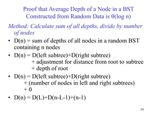
• D(n) = D(L)+D(n-L-1)+(n-1)
• For random data, all subtree sizes equally likely
 
1
0
1
0
1
0
[ ( )] [ ( ) when left tree size is L]
[ ( )] [ ( )] [ ( 1)] ( 1)
2
[ ( )] [ ( )] ( 1)
[ (
Prob(left tree size is L)
1
[ ( ) / ] (lo
)] ( log
g )
)
n
L
n
L
n
L
E D n E D n
n
E D n n
E D n E D L E D n L n
E D n E D L n
n
E D n O n n
O n







     
 
  
 
 




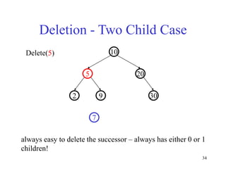
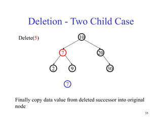
 this looks just like the
Quicksort average case
equation!

26. 26
log
versus
n n
Why is average depth of BST's made from
random inputs different from the average
depth of all pos
log
Because there are more ways to build shallow
trees than d
sible
eep t
BST
ee
?
r
's
n n
s!

27. 27
Random Input vs. Random Trees
Inputs
1,2,3
3,2,1
1,3,2
3,1,2
2,1,3
2,3,1
Trees
For three items, the
shallowest tree is
twice as likely as
any other – effect
grows as n
increases. For n=4,
probability of
getting a shallow
tree > 50%

28. 28
Deletion
20
9
2
15
5
10
30
7 17
Why might deletion be harder than insertion?

29. 29
FindMin/FindMax
Node min(Node root) {
if (root.left == NULL)
return root;
else
return min(root.left);
}
20
9
2
15
5
10
30
7 17
How many children can the min of a node have?

30. 30
Successor
Find the next larger node
in this node’s subtree.
– not next larger in entire
tree
Node succ(Node root) {
if (root.right == NULL)
return NULL;
else
return
min(root.right);
}
20
9
2
15
5
10
30
7 17
How many children can the successor of a node have?

31. 31
Deletion - Leaf Case
20
9
2
15
5
10
30
7 17
Delete(17)

32. 32
Deletion - One Child Case
20
9
2
15
5
10
30
7
Delete(15)

33. 33
Deletion - Two Child Case
30
9
2
20
5
10
7
Delete(5)
replace node with value guaranteed to be between the left and
right subtrees: the successor
Could we have used the predecessor instead?

34. 34
Deletion - Two Child Case
30
9
2
20
5
10
7
Delete(5)
always easy to delete the successor – always has either 0 or 1
children!

35. 35
Deletion - Two Child Case
30
9
2
20
7
10
7
Delete(5)
Finally copy data value from deleted successor into original
node

36. 36
Lazy Deletion
• Instead of physically deleting
nodes, just mark them as
deleted
+ simpler
+ physical deletions done in batches
+ some adds just flip deleted flag
– extra memory for deleted flag
– many lazy deletions slow finds
– some operations may have to be
modified (e.g., min and max)
20
9
2
15
5
10
30
7 17

37. 37
Dictionary Implementations
BST’s looking good for shallow trees, i.e. the depth D is
small (log n), otherwise as bad as a linked list!
unsorted
array
sorted
array
linked
list
BST
insert find +
O(1)
O(n) find +
O(1)
O(Depth)
find O(n) O(log n) O(n) O(Depth)
delete find +
O(1)
O(n) find +
O(1)
O(Depth)

38. 38
CSE 326: Data Structures
Part 3: Trees, continued
Balancing Act
Henry Kautz
Autumn Quarter 2002

39. 39
Beauty is Only (log n) Deep
• Binary Search Trees are fast if they’re shallow
e.g.: complete
• Problems occur when one branch is much
longer than the other
How to capture the notion of a “sort of” complete
tree?

40. 40
Balance
balance = height(left subtree) - height(right subtree)
• convention: height of a “null” subtree is -1
• zero everywhere  perfectly balanced
• small everywhere  balanced enough: (log n)
– Precisely: Maximum depth is 1.44 log n
t
5
6

41. 41
AVL Tree
Dictionary Data Structure
4
12
10
6
2
11
5
8
14
13
7 9
• Binary search tree
properties
• Balance of every node is
-1 b  1
• Tree re-balances itself
after every insert or
delete
15
What is the balance of each node in this tree?

42. 42
AVL Tree Data Structure
15
9
2 12
5
10
20
17
0
0
1
0
0
1 2
3 10
3
data
height
children
30
0

43. 43
Not An AVL Tree
15
9
2 12
5
10
20
17
0
1
2
0
0
1 3
4 10
4
data
height
children
30
0
18
0

44. 44
Bad Case #1
Insert(small)
Insert(middle)
Insert(tall)
T
M
S
0
1
2

45. 45
Single Rotation
T
M
S
0
1
2
M
S T
0
0
1
Basic operation used in AVL trees:
A right child could legally have its
parent as its left child.

46. 46
General Case: Insert Unbalances
a
X
Y
b
Z
h h - 1
h + 1 h - 1
h + 2
a
X
Y
b
Z
h-1 h - 1
h h - 1
h + 1
a
X
Y
b
Z
h
h - 1
h
h - 1
h + 1

47. 47
Properties of General Insert +
Single Rotation
• Restores balance to a lowest point in tree
where imbalance occurs
• After rotation, height of the subtree (in the
example, h+1) is the same as it was before
the insert that imbalanced it
• Thus, no further rotations are needed
anywhere in the tree!

48. 48
Bad Case #2
Insert(small)
Insert(tall)
Insert(middle)
M
T
S
0
1
2
Why won’t a single
rotation (bringing T up to
the top) fix this?

49. 49
Double Rotation
M
S T
0
0
1
M
T
S
0
1
2
T
M
S
0
1
2

50. 50
General Double Rotation
• Initially: insert into X unbalances tree (root height goes to h+3)
• “Zig zag” to pull up c – restores root height to h+2, left subtree
height to h
a
Z
b
W
c
Y
a
Z
b
W
c
Y
h+1
h
h
h
h + 3
h + 2
h
h
h+1
h + 2
h+1
h
X
X

51. 51
Another Double Rotation Case
• Initially: insert into Y unbalances tree (root height goes to h+2)
• “Zig zag” to pull up c – restores root height to h+1, left subtree
height to h
a
Z
b
W
c
Y
a
Z
b
W
c
Y
h+1
h
h
h
h + 3
h + 2
h
h
h+1
h + 2
h+1
h
X
X

52. 52
Insert Algorithm
• Find spot for value
• Hang new node
• Search back up looking for imbalance
• If there is an imbalance:
“outside”: Perform single rotation and exit
“inside”: Perform double rotation and exit

53. 53
AVL Insert Algorithm
Node insert(Comparable x, Node root){
// returns root of revised tree
if ( root == NULL )
return new Node(x);
if (x <= root.key){
root.left = insert( x, root.left );
if (root unbalanced) { rotate... } }
else { // x > root.key
root.right = insert( x, root.right );
if (root unbalanced) { rotate... } }
root.height = max(root.left.height,
root.right.height)+1;
return root;
}

54. 54
Deletion (Really Easy Case)
20
9
2
15
5
10
30
17
3
12
1
0
1
0
0
2 2
3
0
0
Delete(17)

55. 55
Deletion (Pretty Easy Case)
20
9
2
15
5
10
30
17
3
12
1
0
1
0
0
2 2
3
0
0
Delete(15)

56. 56
Deletion (Pretty Easy Case cont.)
20
9
2
17
5
10
30
3
12
1 1
0
0
2 2
3
0
0
Delete(15)

57. 57
Deletion (Hard Case #1)
20
9
2
17
5
10
30
3
12
1 1
0
0
2 2
3
0
0
Delete(12)

58. 58
Single Rotation on Deletion
20
9
2
17
5
10
30
3
1 1
0
2 2
3
0
0
30
9
2
20
5
10
17
3
1 0
0
2 1
3
0
0
What is different about
deletion than insertion?

59. 59
Deletion (Hard Case)
Delete(9)
20
9
2
17
5
10
30
3
12
1 2
2
0
2 3
4
0
33
15
13
0 0
1
0
20
30
12
33
15
13
1
0 0
11
0
18
0

60. 60
Double Rotation on Deletion
2
3
0
20
2
17
5
10
30
12
1 2
2
2 3
4
33
15
13
1
0 0
1
11
0
18
0
20
5
2
17
3
10
30
12
0 2
2
0
1 3
4
33
15
13
1
0 0
1
11
0
18
0
0
Not
finished!

61. 61
Deletion with Propagation
We get to choose whether
to single or double rotate!
20
5
2
17
3
10
30
12
0 2
2
0
1 3
4
33
15
13
1
0 0
1
11
0
18
0
What different
about this case?

62. 62
Propagated Single Rotation
0
30
20
17
33
12
15
13
1
0
5
2
3
10
4
3 2
1 2 1
0 0 0
11
0
20
5
2
17
3
10
30
12
0 2
2
0
1 3
4
33
15
13
1
0
1
11
0
18
0
18
0

63. 63
Propagated Double Rotation
0
17
12
11
5
2
3
10
4
2 3
1 0
0 0
20
5
2
17
3
10
30
12
0 2
2
0
1 3
4
33
15
13
1
0
1
11
0
18
0
15
1
0
20
30
33
1
18
0
13
0
2

64. 64
AVL Deletion Algorithm
• Recursive
1. If at node, delete it
2. Otherwise recurse to
find it in
3. Correct heights
a. If imbalance #1,
single rotate
b. If imbalance #2
(or don’t care),
double rotate
• Iterative
1. Search downward for
node, stacking
parent nodes
2. Delete node
3. Unwind stack,
correcting heights
a. If imbalance #1,
single rotate
b. If imbalance #2
(or don’t care)
double rotate

65. 65
AVL
• Automatically Virtually Leveled
• Architecture for inVisible Leveling
• Articulating Various Lines
• Amortizing? Very Lousy!
• Amazingly Vexing Letters

66. 66
AVL
• Automatically Virtually Leveled
• Architecture for inVisible Leveling
• Articulating Various Lines
• Amortizing? Very Lousy!
• Amazingly Vexing Letters
Adelson-Velskii Landis

67. 67
Pro:
• All operations guaranteed O(log N)
• The height balancing adds no more than a
constant factor to the speed of insertion
Con:
• Space consumed by height field in each node
• Slower than ordinary BST on random data
Can we guarantee O(log N) performance with less
overhead?
Pros and Cons of AVL Trees

68. 68
Splay
Trees
CSE 326: Data Structures
Part 3: Trees, continued

69. 69
Today: Splay Trees
• Fast both in worst-case amortized analysis
and in practice
• Are used in the kernel of NT for keep track of
process information!
• Invented by Sleator and Tarjan (1985)
• Details:
• Weiss 4.5 (basic splay trees)
• 11.5 (amortized analysis)
• 12.1 (better “top down” implementation)

70. 70
Basic Idea
“Blind” rebalancing – no height info kept!
• Worst-case time per operation is O(n)
• Worst-case amortized time is O(log n)
• Insert/find always rotates node to the root!
• Good locality:
– Most commonly accessed keys move high in
tree – become easier and easier to find

71. 71
Idea
17
10
9
2
5
3
You’re forced to make
a really deep access:
Since you’re down there anyway,
fix up a lot of deep nodes!
move n to root by
series of zig-zag
and zig-zig
rotations, followed
by a final single
rotation (zig) if
necessary

72. 72
Zig-Zag*
g
X
p
Y
n
Z
W
*This is just a double rotation
n
Y
g
W
p
Z
X
Helped
Unchanged
Hurt
up 2
down 1
up 1
down 1

73. 73
Zig-Zig
n
Z
Y
p
X
g
W
g
W
X
p
Y
n
Z

74. 74
Why Splaying Helps
• Node n and its children are always helped (raised)
• Except for last step, nodes that are hurt by a zig-
zag or zig-zig are later helped by a rotation higher
up the tree!
• Result:
– shallow nodes may increase depth by one or two
– helped nodes decrease depth by a large amount
• If a node n on the access path is at depth d before
the splay, it’s at about depth d/2 after the splay
– Exceptions are the root, the child of the root, and the
node splayed

75. 75
Splaying Example
2
1
3
4
5
6
Find(6)
2
1
3
6
5
4
zig-zig

76. 76
Still Splaying 6
zig-zig
2
1
3
6
5
4
1
6
3
2 5
4

77. 77
Almost There, Stay on Target
zig
1
6
3
2 5
4
6
1
3
2 5
4

78. 78
Splay Again
Find(4)
zig-zag
6
1
3
2 5
4
6
1
4
3 5
2

79. 79
Example Splayed Out
zig-zag
6
1
4
3 5
2
6
1
4
3 5
2

80. 80
Locality
• “Locality” – if an item is accessed, it is likely to
be accessed again soon
– Why?
• Assume m  n access in a tree of size n
– Total worst case time is O(m log n)
– O(log n) per access amortized time
• Suppose only k distinct items are accessed in the
m accesses.
– Time is O(n log n + m log k )
– Compare with O( m log n ) for AVL tree
getting those k items
near root
those k items are all at
the top of the tree

81. 81
Splay Operations: Insert
• To insert, could do an ordinary BST insert
– but would not fix up tree
– A BST insert followed by a find (splay)?
• Better idea: do the splay before the insert!
• How?

82. 82
Split
Split(T, x) creates two BST’s L and R:
– All elements of T are in either L or R
– All elements in L are  x
– All elements in R are  x
– L and R share no elements
Then how do we do the insert?

83. 83
Split
Split(T, x) creates two BST’s L and R:
– All elements of T are in either L or R
– All elements in L are  x
– All elements in R are > x
– L and R share no elements
Then how do we do the insert?
Insert as root, with children L and R

84. 84
Splitting in Splay Trees
• How can we split?
– We have the splay operation
– We can find x or the parent of where x would
be if we were to insert it as an ordinary BST
– We can splay x or the parent to the root
– Then break one of the links from the root to a
child

85. 85
Split
split(x)
T L R
splay
OR
L R L R
 x > x
> x < x
could be x, or
what would
have been the
parent of x
if root is  x
if root is > x

86. 86
Back to Insert
split(x)
L R
x
L R
> x
 x
Insert(x):
Split on x
Join subtrees using x as root

87. 87
Insert Example
9
1
6
4 7
2
Insert(5)
split(5)
9
6
7
1
4
2
1
4
2
9
6
7
1
4
2
9
6
7
5

88. 88
Splay Operations: Delete
find(x)
L R
x
L R
> x
< x
delete x
Now what?

89. 89
Join
• Join(L, R): given two trees such that L < R,
merge them
• Splay on the maximum element in L then
attach R
L R R
splay L

90. 90
Delete Completed
T
find(x)
L R
x
L R
> x
< x
delete x
T - x
Join(L,R)

91. 91
Delete Example
9
1
6
4 7
2
Delete(4)
find(4)
9
6
7
1
4
2
1
2
9
6
7
Find max
2
1
9
6
7
2
1
9
6
7

92. 92
Splay Trees, Summary
• Splay trees are arguably the most practical
kind of self-balancing trees
• If number of finds is much larger than n,
then locality is crucial!
– Example: word-counting
• Also supports efficient Split and Join
operations – useful for other tasks
– E.g., range queries