Contoh materi searching MUDENG

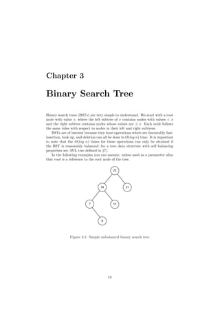
1. Chapter 3
Binary Search Tree
Binary search trees (BSTs) are very simple to understand. We start with a root
node with value x, where the left subtree of x contains nodes with values < x
and the right subtree contains nodes whose values are ≥ x. Each node follows
the same rules with respect to nodes in their left and right subtrees.
BSTs are of interest because they have operations which are favourably fast:
insertion, look up, and deletion can all be done in O(log n) time. It is important
to note that the O(log n) times for these operations can only be attained if
the BST is reasonably balanced; for a tree data structure with self balancing
properties see AVL tree defined in §7).
In the following examples you can assume, unless used as a parameter alias
that root is a reference to the root node of the tree.
!
!
% %
'
Figure 3.1: Simple unbalanced binary search tree
19

2. CHAPTER 3. BINARY SEARCH TREE 20
3.1 Insertion
As mentioned previously insertion is an O(log n) operation provided that the
tree is moderately balanced.
1) algorithm Insert(value)
2) Pre: value has passed custom type checks for type T
3) Post: value has been placed in the correct location in the tree
4) if root = ∅
5) root ← node(value)
6) else
7) InsertNode(root, value)
8) end if
9) end Insert
1) algorithm InsertNode(current, value)
2) Pre: current is the node to start from
3) Post: value has been placed in the correct location in the tree
4) if value current.Value
5) if current.Left = ∅
6) current.Left ← node(value)
7) else
8) InsertNode(current.Left, value)
9) end if
10) else
11) if current.Right = ∅
12) current.Right ← node(value)
13) else
14) InsertNode(current.Right, value)
15) end if
16) end if
17) end InsertNode
The insertion algorithm is split for a good reason. The first algorithm (non-
recursive) checks a very core base case - whether or not the tree is empty. If
the tree is empty then we simply create our root node and finish. In all other
cases we invoke the recursive InsertNode algorithm which simply guides us to
the first appropriate place in the tree to put value. Note that at each stage we
perform a binary chop: we either choose to recurse into the left subtree or the
right by comparing the new value with that of the current node. For any totally
ordered type, no value can simultaneously satisfy the conditions to place it in
both subtrees.

3. CHAPTER 3. BINARY SEARCH TREE 21
3.2 Searching
Searching a BST is even simpler than insertion. The pseudocode is self-explanatory
but we will look briefly at the premise of the algorithm nonetheless.
We have talked previously about insertion, we go either left or right with the
right subtree containing values that are ≥ x where x is the value of the node
we are inserting. When searching the rules are made a little more atomic and
at any one time we have four cases to consider:
1. the root = ∅ in which case value is not in the BST; or
2. root.Value = value in which case value is in the BST; or
3. value root.Value, we must inspect the left subtree of root for value; or
4. value root.Value, we must inspect the right subtree of root for value.
1) algorithm Contains(root, value)
2) Pre: root is the root node of the tree, value is what we would like to locate
3) Post: value is either located or not
4) if root = ∅
5) return false
6) end if
7) if root.Value = value
8) return true
9) else if value root.Value
10) return Contains(root.Left, value)
11) else
12) return Contains(root.Right, value)
13) end if
14) end Contains

4. CHAPTER 3. BINARY SEARCH TREE 22
3.3 Deletion
Removing a node from a BST is fairly straightforward, with four cases to con-
sider:
1. the value to remove is a leaf node; or
2. the value to remove has a right subtree, but no left subtree; or
3. the value to remove has a left subtree, but no right subtree; or
4. the value to remove has both a left and right subtree in which case we
promote the largest value in the left subtree.
There is also an implicit fifth case whereby the node to be removed is the
only node in the tree. This case is already covered by the first, but should be
noted as a possibility nonetheless.
Of course in a BST a value may occur more than once. In such a case the
first occurrence of that value in the BST will be removed.
23
14 31
7
9#1: Leaf Node
#2: Right subtree
no left subtree
#3: Left subtree
no right subtree
#4: Right subtree
and left subtree
Figure 3.2: binary search tree deletion cases
The Remove algorithm given below relies on two further helper algorithms
named FindParent, and FindNode which are described in §3.4 and §3.5 re-
spectively.

5. CHAPTER 3. BINARY SEARCH TREE 23
1) algorithm Remove(value)
2) Pre: value is the value of the node to remove, root is the root node of the BST
3) Count is the number of items in the BST
3) Post: node with value is removed if found in which case yields true, otherwise false
4) nodeToRemove ← FindNode(value)
5) if nodeToRemove = ∅
6) return false // value not in BST
7) end if
8) parent ← FindParent(value)
9) if Count = 1
10) root ← ∅ // we are removing the only node in the BST
11) else if nodeToRemove.Left = ∅ and nodeToRemove.Right = null
12) // case #1
13) if nodeToRemove.Value parent.Value
14) parent.Left ← ∅
15) else
16) parent.Right ← ∅
17) end if
18) else if nodeToRemove.Left = ∅ and nodeToRemove.Right = ∅
19) // case # 2
20) if nodeToRemove.Value parent.Value
21) parent.Left ← nodeToRemove.Right
22) else
23) parent.Right ← nodeToRemove.Right
24) end if
25) else if nodeToRemove.Left = ∅ and nodeToRemove.Right = ∅
26) // case #3
27) if nodeToRemove.Value parent.Value
28) parent.Left ← nodeToRemove.Left
29) else
30) parent.Right ← nodeToRemove.Left
31) end if
32) else
33) // case #4
34) largestV alue ← nodeToRemove.Left
35) while largestV alue.Right = ∅
36) // find the largest value in the left subtree of nodeToRemove
37) largestV alue ← largestV alue.Right
38) end while
39) // set the parents’ Right pointer of largestV alue to ∅
40) FindParent(largestV alue.Value).Right ← ∅
41) nodeToRemove.Value ← largestV alue.Value
42) end if
43) Count ← Count −1
44) return true
45) end Remove

6. CHAPTER 3. BINARY SEARCH TREE 24
3.4 Finding the parent of a given node
The purpose of this algorithm is simple - to return a reference (or pointer) to
the parent node of the one with the given value. We have found that such an
algorithm is very useful, especially when performing extensive tree transforma-
tions.
1) algorithm FindParent(value, root)
2) Pre: value is the value of the node we want to find the parent of
3) root is the root node of the BST and is ! = ∅
4) Post: a reference to the parent node of value if found; otherwise ∅
5) if value = root.Value
6) return ∅
7) end if
8) if value root.Value
9) if root.Left = ∅
10) return ∅
11) else if root.Left.Value = value
12) return root
13) else
14) return FindParent(value, root.Left)
15) end if
16) else
17) if root.Right = ∅
18) return ∅
19) else if root.Right.Value = value
20) return root
21) else
22) return FindParent(value, root.Right)
23) end if
24) end if
25) end FindParent
A special case in the above algorithm is when the specified value does not
exist in the BST, in which case we return ∅. Callers to this algorithm must take
account of this possibility unless they are already certain that a node with the
specified value exists.
3.5 Attaining a reference to a node
This algorithm is very similar to §3.4, but instead of returning a reference to the
parent of the node with the specified value, it returns a reference to the node
itself. Again, ∅ is returned if the value isn’t found.

7. CHAPTER 3. BINARY SEARCH TREE 25
1) algorithm FindNode(root, value)
2) Pre: value is the value of the node we want to find the parent of
3) root is the root node of the BST
4) Post: a reference to the node of value if found; otherwise ∅
5) if root = ∅
6) return ∅
7) end if
8) if root.Value = value
9) return root
10) else if value root.Value
11) return FindNode(root.Left, value)
12) else
13) return FindNode(root.Right, value)
14) end if
15) end FindNode
Astute readers will have noticed that the FindNode algorithm is exactly the
same as the Contains algorithm (defined in §3.2) with the modification that
we are returning a reference to a node not true or false. Given FindNode,
the easiest way of implementing Contains is to call FindNode and compare the
return value with ∅.
3.6 Finding the smallest and largest values in
the binary search tree
To find the smallest value in a BST you simply traverse the nodes in the left
subtree of the BST always going left upon each encounter with a node, termi-
nating when you find a node with no left subtree. The opposite is the case when
finding the largest value in the BST. Both algorithms are incredibly simple, and
are listed simply for completeness.
The base case in both FindMin, and FindMax algorithms is when the Left
(FindMin), or Right (FindMax) node references are ∅ in which case we have
reached the last node.
1) algorithm FindMin(root)
2) Pre: root is the root node of the BST
3) root = ∅
4) Post: the smallest value in the BST is located
5) if root.Left = ∅
6) return root.Value
7) end if
8) FindMin(root.Left)
9) end FindMin

8. CHAPTER 3. BINARY SEARCH TREE 26
1) algorithm FindMax(root)
2) Pre: root is the root node of the BST
3) root = ∅
4) Post: the largest value in the BST is located
5) if root.Right = ∅
6) return root.Value
7) end if
8) FindMax(root.Right)
9) end FindMax
3.7 Tree Traversals
There are various strategies which can be employed to traverse the items in a
tree; the choice of strategy depends on which node visitation order you require.
In this section we will touch on the traversals that DSA provides on all data
structures that derive from BinarySearchTree.
3.7.1 Preorder
When using the preorder algorithm, you visit the root first, then traverse the left
subtree and finally traverse the right subtree. An example of preorder traversal
is shown in Figure 3.3.
1) algorithm Preorder(root)
2) Pre: root is the root node of the BST
3) Post: the nodes in the BST have been visited in preorder
4) if root = ∅
5) yield root.Value
6) Preorder(root.Left)
7) Preorder(root.Right)
8) end if
9) end Preorder
3.7.2 Postorder
This algorithm is very similar to that described in §3.7.1, however the value
of the node is yielded after traversing both subtrees. An example of postorder
traversal is shown in Figure 3.4.
1) algorithm Postorder(root)
2) Pre: root is the root node of the BST
3) Post: the nodes in the BST have been visited in postorder
4) if root = ∅
5) Postorder(root.Left)
6) Postorder(root.Right)
7) yield root.Value
8) end if
9) end Postorder

9. CHAPTER 3. BINARY SEARCH TREE 27
!
!
% %
'
!
!
%
'
!
!
%
'
!
!
%
'
!
!
%
'
!
!
%
'
= ?
@ A B
% %
% % %
Figure 3.3: Preorder visit binary search tree example

10. CHAPTER 3. BINARY SEARCH TREE 28
!
!
% %
'
!
!
%
'
!
!
%
'
!
!
%
'
!
!
%
'
!
!
%
'
= ?
@ A B
% %
% % %
Figure 3.4: Postorder visit binary search tree example

11. CHAPTER 3. BINARY SEARCH TREE 29
3.7.3 Inorder
Another variation of the algorithms defined in §3.7.1 and §3.7.2 is that of inorder
traversal where the value of the current node is yielded in between traversing
the left subtree and the right subtree. An example of inorder traversal is shown
in Figure 3.5.
!
!
% %
'
!
!
%
'
!
!
%
'
!
!
%
'
!
!
%
'
!
!
%
'
= ?
@ A B
% %
% % %
Figure 3.5: Inorder visit binary search tree example
1) algorithm Inorder(root)
2) Pre: root is the root node of the BST
3) Post: the nodes in the BST have been visited in inorder
4) if root = ∅
5) Inorder(root.Left)
6) yield root.Value
7) Inorder(root.Right)
8) end if
9) end Inorder
One of the beauties of inorder traversal is that values are yielded in their
comparison order. In other words, when traversing a populated BST with the
inorder strategy, the yielded sequence would have property xi ≤ xi+1∀i.

12. CHAPTER 3. BINARY SEARCH TREE 30
3.7.4 Breadth First
Traversing a tree in breadth first order yields the values of all nodes of a par-
ticular depth in the tree before any deeper ones. In other words, given a depth
d we would visit the values of all nodes at d in a left to right fashion, then we
would proceed to d + 1 and so on until we hade no more nodes to visit. An
example of breadth first traversal is shown in Figure 3.6.
Traditionally breadth first traversal is implemented using a list (vector, re-
sizeable array, etc) to store the values of the nodes visited in breadth first order
and then a queue to store those nodes that have yet to be visited.
!
!
% %
'
!
!
%
'
!
!
%
'
!
!
%
'
!
!
%
'
!
!
%
'
= ?
@ A B
% %
% % %
Figure 3.6: Breadth First visit binary search tree example

13. CHAPTER 3. BINARY SEARCH TREE 31
1) algorithm BreadthFirst(root)
2) Pre: root is the root node of the BST
3) Post: the nodes in the BST have been visited in breadth first order
4) q ← queue
5) while root = ∅
6) yield root.Value
7) if root.Left = ∅
8) q.Enqueue(root.Left)
9) end if
10) if root.Right = ∅
11) q.Enqueue(root.Right)
12) end if
13) if !q.IsEmpty()
14) root ← q.Dequeue()
15) else
16) root ← ∅
17) end if
18) end while
19) end BreadthFirst
3.8 Summary
A binary search tree is a good solution when you need to represent types that are
ordered according to some custom rules inherent to that type. With logarithmic
insertion, lookup, and deletion it is very effecient. Traversal remains linear, but
there are many ways in which you can visit the nodes of a tree. Trees are
recursive data structures, so typically you will find that many algorithms that
operate on a tree are recursive.
The run times presented in this chapter are based on a pretty big assumption
- that the binary search tree’s left and right subtrees are reasonably balanced.
We can only attain logarithmic run times for the algorithms presented earlier
when this is true. A binary search tree does not enforce such a property, and
the run times for these operations on a pathologically unbalanced tree become
linear: such a tree is effectively just a linked list. Later in §7 we will examine
an AVL tree that enforces self-balancing properties to help attain logarithmic
run times.

14. Chapter 4
Heap
A heap can be thought of as a simple tree data structure, however a heap usually
employs one of two strategies:
1. min heap; or
2. max heap
Each strategy determines the properties of the tree and its values. If you
were to choose the min heap strategy then each parent node would have a value
that is ≤ than its children. For example, the node at the root of the tree will
have the smallest value in the tree. The opposite is true for the max heap
strategy. In this book you should assume that a heap employs the min heap
strategy unless otherwise stated.
Unlike other tree data structures like the one defined in §3 a heap is generally
implemented as an array rather than a series of nodes which each have refer-
ences to other nodes. The nodes are conceptually the same, however, having at
most two children. Figure 4.1 shows how the tree (not a heap data structure)
(12 7(3 2) 6(9 )) would be represented as an array. The array in Figure 4.1 is a
result of simply adding values in a top-to-bottom, left-to-right fashion. Figure
4.2 shows arrows to the direct left and right child of each value in the array.
This chapter is very much centred around the notion of representing a tree as
an array and because this property is key to understanding this chapter Figure
4.3 shows a step by step process to represent a tree data structure as an array.
In Figure 4.3 you can assume that the default capacity of our array is eight.
Using just an array is often not sufficient as we have to be up front about the
size of the array to use for the heap. Often the run time behaviour of a program
can be unpredictable when it comes to the size of its internal data structures,
so we need to choose a more dynamic data structure that contains the following
properties:
1. we can specify an initial size of the array for scenarios where we know the
upper storage limit required; and
2. the data structure encapsulates resizing algorithms to grow the array as
required at run time
32

15. CHAPTER 4. HEAP 33
Figure 4.1: Array representation of a simple tree data structure
Figure 4.2: Direct children of the nodes in an array representation of a tree data
structure
1. Vector
2. ArrayList
3. List
Figure 4.1 does not specify how we would handle adding null references to
the heap. This varies from case to case; sometimes null values are prohibited
entirely; in other cases we may treat them as being smaller than any non-null
value, or indeed greater than any non-null value. You will have to resolve this
ambiguity yourself having studied your requirements. For the sake of clarity we
will avoid the issue by prohibiting null values.
Because we are using an array we need some way to calculate the index of a
parent node, and the children of a node. The required expressions for this are
defined as follows for a node at index:
1. (index − 1)/2 (parent index)
2. 2 ∗ index + 1 (left child)
3. 2 ∗ index + 2 (right child)
In Figure 4.4 a) represents the calculation of the right child of 12 (2 ∗ 0 + 2);
and b) calculates the index of the parent of 3 ((3 − 1)/2).
4.1 Insertion
Designing an algorithm for heap insertion is simple, but we must ensure that
heap order is preserved after each insertion. Generally this is a post-insertion
operation. Inserting a value into the next free slot in an array is simple: we just
need to keep track of the next free index in the array as a counter, and increment
it after each insertion. Inserting our value into the heap is the first part of the
algorithm; the second is validating heap order. In the case of min-heap ordering
this requires us to swap the values of a parent and its child if the value of the
child is the value of its parent. We must do this for each subtree containing
the value we just inserted.

16. CHAPTER 4. HEAP 34
Figure 4.3: Converting a tree data structure to its array counterpart

17. CHAPTER 4. HEAP 35
Figure 4.4: Calculating node properties
The run time efficiency for heap insertion is O(log n). The run time is a
by product of verifying heap order as the first part of the algorithm (the actual
insertion into the array) is O(1).
Figure 4.5 shows the steps of inserting the values 3, 9, 12, 7, and 1 into a
min-heap.

18. CHAPTER 4. HEAP 36
Figure 4.5: Inserting values into a min-heap

19. CHAPTER 4. HEAP 37
1) algorithm Add(value)
2) Pre: value is the value to add to the heap
3) Count is the number of items in the heap
4) Post: the value has been added to the heap
5) heap[Count] ← value
6) Count ← Count +1
7) MinHeapify()
8) end Add
1) algorithm MinHeapify()
2) Pre: Count is the number of items in the heap
3) heap is the array used to store the heap items
4) Post: the heap has preserved min heap ordering
5) i ← Count −1
6) while i 0 and heap[i] heap[(i − 1)/2]
7) Swap(heap[i], heap[(i − 1)/2]
8) i ← (i − 1)/2
9) end while
10) end MinHeapify
The design of the MaxHeapify algorithm is very similar to that of the Min-
Heapify algorithm, the only difference is that the operator in the second
condition of entering the while loop is changed to .
4.2 Deletion
Just as for insertion, deleting an item involves ensuring that heap ordering is
preserved. The algorithm for deletion has three steps:
1. find the index of the value to delete
2. put the last value in the heap at the index location of the item to delete
3. verify heap ordering for each subtree which used to include the value

20. CHAPTER 4. HEAP 38
1) algorithm Remove(value)
2) Pre: value is the value to remove from the heap
3) left, and right are updated alias’ for 2 ∗ index + 1, and 2 ∗ index + 2 respectively
4) Count is the number of items in the heap
5) heap is the array used to store the heap items
6) Post: value is located in the heap and removed, true; otherwise false
7) // step 1
8) index ← FindIndex(heap, value)
9) if index 0
10) return false
11) end if
12) Count ← Count −1
13) // step 2
14) heap[index] ← heap[Count]
15) // step 3
16) while left Count and heap[index] heap[left] or heap[index] heap[right]
17) // promote smallest key from subtree
18) if heap[left] heap[right]
19) Swap(heap, left, index)
20) index ← left
21) else
22) Swap(heap, right, index)
23) index ← right
24) end if
25) end while
26) return true
27) end Remove
Figure 4.6 shows the Remove algorithm visually, removing 1 from a heap
containing the values 1, 3, 9, 12, and 13. In Figure 4.6 you can assume that we
have specified that the backing array of the heap should have an initial capacity
of eight.
Please note that in our deletion algorithm that we don’t default the removed
value in the heap array. If you are using a heap for reference types, i.e. objects
that are allocated on a heap you will want to free that memory. This is important
in both unmanaged, and managed languages. In the latter we will want to null
that empty hole so that the garbage collector can reclaim that memory. If we
were to not null that hole then the object could still be reached and thus won’t
be garbage collected.
4.3 Searching
Searching a heap is merely a matter of traversing the items in the heap array
sequentially, so this operation has a run time complexity of O(n). The search
can be thought of as one that uses a breadth first traversal as defined in §3.7.4
to visit the nodes within the heap to check for the presence of a specified item.

21. CHAPTER 4. HEAP 39
Figure 4.6: Deleting an item from a heap

22. CHAPTER 4. HEAP 40
1) algorithm Contains(value)
2) Pre: value is the value to search the heap for
3) Count is the number of items in the heap
4) heap is the array used to store the heap items
5) Post: value is located in the heap, in which case true; otherwise false
6) i ← 0
7) while i Count and heap[i] = value
8) i ← i + 1
9) end while
10) if i Count
11) return true
12) else
13) return false
14) end if
15) end Contains
The problem with the previous algorithm is that we don’t take advantage
of the properties in which all values of a heap hold, that is the property of the
heap strategy being used. For instance if we had a heap that didn’t contain the
value 4 we would have to exhaust the whole backing heap array before we could
determine that it wasn’t present in the heap. Factoring in what we know about
the heap we can optimise the search algorithm by including logic which makes
use of the properties presented by a certain heap strategy.
Optimising to deterministically state that a value is in the heap is not that
straightforward, however the problem is a very interesting one. As an example
consider a min-heap that doesn’t contain the value 5. We can only rule that the
value is not in the heap if 5 the parent of the current node being inspected
and the current node being inspected ∀ nodes at the current level we are
traversing. If this is the case then 5 cannot be in the heap and so we can
provide an answer without traversing the rest of the heap. If this property is
not satisfied for any level of nodes that we are inspecting then the algorithm
will indeed fall back to inspecting all the nodes in the heap. The optimisation
that we present can be very common and so we feel that the extra logic within
the loop is justified to prevent the expensive worse case run time.
The following algorithm is specifically designed for a min-heap. To tailor the
algorithm for a max-heap the two comparison operations in the else if condition
within the inner while loop should be flipped.

23. CHAPTER 4. HEAP 41
1) algorithm Contains(value)
2) Pre: value is the value to search the heap for
3) Count is the number of items in the heap
4) heap is the array used to store the heap items
5) Post: value is located in the heap, in which case true; otherwise false
6) start ← 0
7) nodes ← 1
8) while start Count
9) start ← nodes − 1
10) end ← nodes + start
11) count ← 0
12) while start Count and start end
13) if value = heap[start]
14) return true
15) else if value Parent(heap[start]) and value heap[start]
16) count ← count + 1
17) end if
18) start ← start + 1
19) end while
20) if count = nodes
21) return false
22) end if
23) nodes ← nodes ∗ 2
24) end while
25) return false
26) end Contains
The new Contains algorithm determines if the value is not in the heap by
checking whether count = nodes. In such an event where this is true then we
can confirm that ∀ nodes n at level i : value Parent(n), value n thus there
is no possible way that value is in the heap. As an example consider Figure 4.7.
If we are searching for the value 10 within the min-heap displayed it is obvious
that we don’t need to search the whole heap to determine 9 is not present. We
can verify this after traversing the nodes in the second level of the heap as the
previous expression defined holds true.
4.4 Traversal
As mentioned in §4.3 traversal of a heap is usually done like that of any other
array data structure which our heap implementation is based upon. As a result
you traverse the array starting at the initial array index (0 in most languages)
and then visit each value within the array until you have reached the upper
bound of the heap. You will note that in the search algorithm that we use Count
as this upper bound rather than the actual physical bound of the allocated
array. Count is used to partition the conceptual heap from the actual array
implementation of the heap: we only care about the items in the heap, not the
whole array—the latter may contain various other bits of data as a result of
heap mutation.

24. CHAPTER 4. HEAP 42
Figure 4.7: Determining 10 is not in the heap after inspecting the nodes of Level
2
Figure 4.8: Living and dead space in the heap backing array
If you have followed the advice we gave in the deletion algorithm then a
heap that has been mutated several times will contain some form of default
value for items no longer in the heap. Potentially you will have at most
LengthOf(heapArray) − Count garbage values in the backing heap array data
structure. The garbage values of course vary from platform to platform. To
make things simple the garbage value of a reference type will be simple ∅ and 0
for a value type.
Figure 4.8 shows a heap that you can assume has been mutated many times.
For this example we can further assume that at some point the items in indexes
3 − 5 actually contained references to live objects of type T. In Figure 4.8
subscript is used to disambiguate separate objects of T.
From what you have read thus far you will most likely have picked up that
traversing the heap in any other order would be of little benefit. The heap
property only holds for the subtree of each node and so traversing a heap in
any other fashion requires some creative intervention. Heaps are not usually
traversed in any other way than the one prescribed previously.
4.5 Summary
Heaps are most commonly used to implement priority queues (see §6.2 for a
sample implementation) and to facilitate heap sort. As discussed in both the
insertion §4.1 and deletion §4.2 sections a heap maintains heap order according
to the selected ordering strategy. These strategies are referred to as min-heap,

25. CHAPTER 4. HEAP 43
and max heap. The former strategy enforces that the value of a parent node is
less than that of each of its children, the latter enforces that the value of the
parent is greater than that of each of its children.
When you come across a heap and you are not told what strategy it enforces
you should assume that it uses the min-heap strategy. If the heap can be
configured otherwise, e.g. to use max-heap then this will often require you to
state this explicitly. The heap abides progressively to a strategy during the
invocation of the insertion, and deletion algorithms. The cost of such a policy is
that upon each insertion and deletion we invoke algorithms that have logarithmic
run time complexities. While the cost of maintaining the strategy might not
seem overly expensive it does still come at a price. We will also have to factor
in the cost of dynamic array expansion at some stage. This will occur if the
number of items within the heap outgrows the space allocated in the heap’s
backing array. It may be in your best interest to research a good initial starting
size for your heap array. This will assist in minimising the impact of dynamic
array resizing.

26. Chapter 10
Searching
10.1 Sequential Search
A simple algorithm that search for a specific item inside a list. It operates
looping on each element O(n) until a match occurs or the end is reached.
1) algorithm SequentialSearch(list, item)
2) Pre: list = ∅
3) Post: return index of item if found, otherwise −1
4) index ← 0
5) while index list.Count and list[index] = item
6) index ← index + 1
7) end while
8) if index list.Count and list[index] = item
9) return index
10) end if
11) return −1
12) end SequentialSearch
10.2 Probability Search
Probability search is a statistical sequential searching algorithm. In addition to
searching for an item, it takes into account its frequency by swapping it with
it’s predecessor in the list. The algorithm complexity still remains at O(n) but
in a non-uniform items search the more frequent items are in the first positions,
reducing list scanning time.
Figure 10.1 shows the resulting state of a list after searching for two items,
notice how the searched items have had their search probability increased after
each search operation respectively.
76

27. CHAPTER 10. SEARCHING 77
Figure 10.1: a) Search(12), b) Search(101)
1) algorithm ProbabilitySearch(list, item)
2) Pre: list = ∅
3) Post: a boolean indicating where the item is found or not;
in the former case swap founded item with its predecessor
4) index ← 0
5) while index list.Count and list[index] = item
6) index ← index + 1
7) end while
8) if index ≥ list.Count or list[index] = item
9) return false
10) end if
11) if index 0
12) Swap(list[index], list[index − 1])
13) end if
14) return true
15) end ProbabilitySearch
10.3 Summary
In this chapter we have presented a few novel searching algorithms. We have
presented more efficient searching algorithms earlier on, like for instance the
logarithmic searching algorithm that AVL and BST tree’s use (defined in §3.2).
We decided not to cover a searching algorithm known as binary chop (another
name for binary search, binary chop usually refers to its array counterpart) as

28. CHAPTER 10. SEARCHING 78
the reader has already seen such an algorithm in §3.
Searching algorithms and their efficiency largely depends on the underlying
data structure being used to store the data. For instance it is quicker to deter-
mine whether an item is in a hash table than it is an array, similarly it is quicker
to search a BST than it is a linked list. If you are going to search for data fairly
often then we strongly advise that you sit down and research the data structures
available to you. In most cases using a list or any other primarily linear data
structure is down to lack of knowledge. Model your data and then research the
data structures that best fit your scenario.