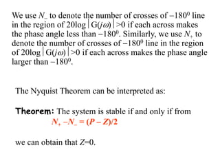
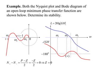
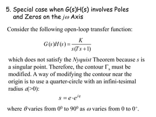
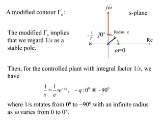
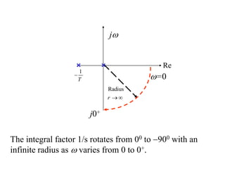
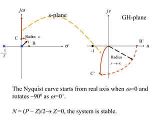
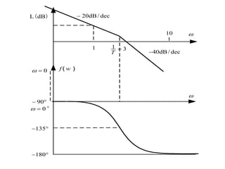
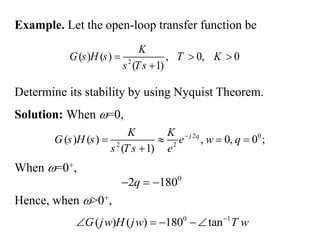
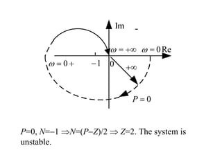
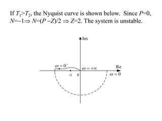
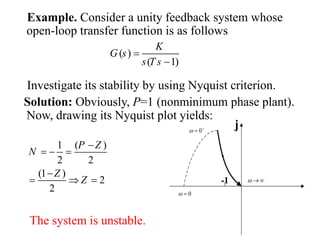
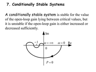
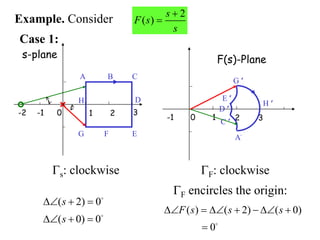
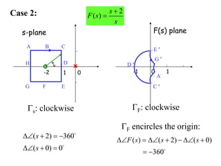
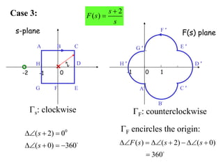
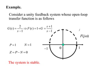
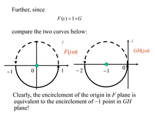
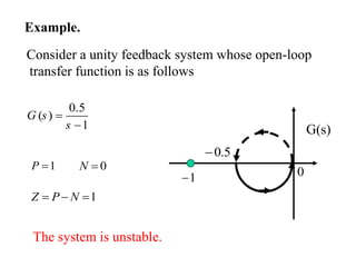
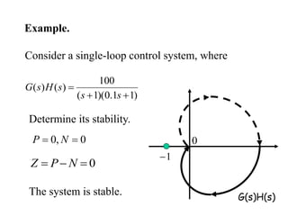
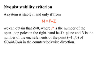
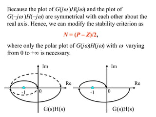
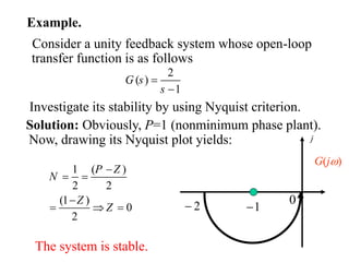
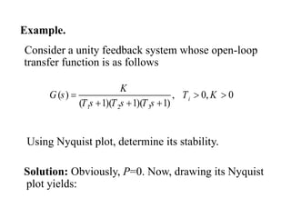
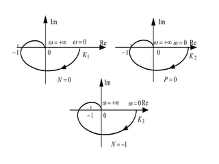
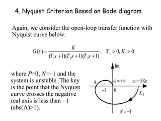
The document discusses the Nyquist stability criterion, which determines the stability of a closed-loop system from its open-loop frequency response and poles. It does not require determining the closed-loop poles. The criterion uses the open-loop transfer function G(s)H(s) and investigates how it maps the Nyquist contour in the s-plane to the F(s)-plane. If the number of encirclements of the origin is equal to the number of open-loop poles, the system is stable. The document provides examples of applying the criterion to various open-loop transfer functions. It also describes interpreting the criterion using the Bode diagram by examining where the phase crosses -180 degrees.

1. 7-4 Nyquist Stability
Criterion

2. 1. Introduction to Nyquist stability criterion
The Nyquist stability criterion determines the stability
of a closed-loop system from its open-loop frequency
response and open-loop poles, and there is no need for
actually determining the closed-loop poles.
To determine the stability of a closed-loop system, one
must investigate the closed-loop characteristic equation
of the system.

3. )
(s
G
)
(s
H
We consider the following typical closed-loop system:
From the above diagram, we have
( )
( )
1 ( ) ( )
G s
s
G s H s
 

1 2
1 2
( ) ( )
( ) : , ( ) :
( ) ( )
N s N s
G s H s
D s D s
 
where
( ) 1 ( ) ( )
F s G s H s
 
We define

4. which is also called the characteristic equation of the
closed-loop system and will play an important role in
stability analysis. In fact, we have
1 2 1 2
1 2
( ) ( ) ( ) ( )
( )
( ) ( )
D s D s N s N s
F s
D s D s


Further, we assume that deg(N1N2)<deg(D1D2), which
implies that both the denominator and nominator
polynomials of F(s) have the same degree.

5. 2. Preliminary Study
Consider, for example, the following open-loop transfer
function:
2
( ) ( )
1
G s H s
s


1
( ) 1 ( ) ( ) ( )
1
s
F s G s H s F s
s

   

whose closed-loop characteristic equation is
which is analytic everywhere except at its singular
points. For each point analytic in s plane, F(s) maps
the point into F(s) plane. For example,
s=2+j:F(s)=2j.
Further, we have the following conclusion:

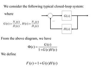
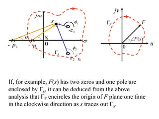
6. Conformal mapping: For any given continuous closed
path in the s plane that does not go through any singular
points, there corresponds a closed curve in the F(s) plane.
s-plane F(s) plane
j

s
[ ]
0
 s
1
s
2
s
3
s
F s
[ ( )]
Im
Re
0
 F
1
F s
( )
2
F s
( )
3
F s
( )

7. 0
-2 -1 1 2 3
s-plane
A B C
F
G
D
E
H
s: clockwise
1
-1 0 2 3
F(s)-Plane
A‫׳‬
C ‫׳‬
G ‫׳‬
D ‫׳‬
E ‫׳‬ H ‫׳‬
F: clockwise
2
( )
s
F s
s


Example. Consider
( ) ( 2) ( 0)
0
F s s s
      

F encircles the origin:
( 2) 0
( 0) 0
  
  
s
s
Case 1:

8. -2 1 0
s-plane
A B C
F
G
D
E
H
s: clockwise
1
-1 0
F(s) plane
A‫׳‬
C ‫׳‬
G ‫׳‬
D ‫׳‬
E ‫׳‬
F: clockwise
2
( )
s
F s
s


( ) ( 2) ( 0)
360
F s s s
      
 
F encircles the origin:
( 2) 360
( 0) 0
   
  
s
s
Case 2:

9. 2
( )
s
F s
s


-2 -1 0
s-plane
A B C
F
G
D
E
H
s: clockwise
1
-1 0
F(s) plane
A‫׳‬ C ‫׳‬
H ‫׳‬ D ‫׳‬
E ‫׳‬
B‫׳‬
F ‫׳‬
G ‫׳‬
F: counterclockwise
( ) ( 2) ( 0)
360
F s s s
      

F encircles the origin:
0
( 2) 0
( 0) 360
  
   
s
s
Case 3:

10. 2
( )
s
F s
s


Case 4:
It can be verified that when s encloses both the pole and
zero in the clockwise direction, the number of the F
encircles the origin is 1+1=0.

11. 1
-z
2
z
1
p
-
2
p
- 0
s 1

2

2
 1



j
0
F
)
(s
F

u
jv
S

F

If, for example, F(s) has two zeros and one pole are
enclosed by s, it can be deduced from the above
analysis that F encircles the origin of F plane one time
in the clockwise direction as s traces out s.

12. Mapping theorem (The principle of argument)
Let F(s) be a ratio of two polynomials in s. Let P be the
number of poles and Z be the number of zeros of F(s)
that lie inside a closed contour s, which does not pass
through any poles and zeros of F(s).
Then the s in the s-plane is mapped into the F(s) plane
as a closed curve, F. The total number N of
counterclockwise encirclements of the origin of the
F(s), as s traces out s in the clockwise direction, is
equal to
N=PZ

13. 3.The Nyquist Stability Criterion
)
(s
G
)
(s
H
1 2 1 2
1 2
( ) ( ) ( ) ( )
( )
( ) ( )
=
D s D s N s N s
F s
D s D s


closed -loop characteristic equation
open -loop characteristic equation
For a stable system, all the zeros of F(s) must lie in the
left-half s-plane.

14. Therefore, we choose a contour s, say, Nyquist path, in
the s-plane that encloses the entire right-half s-plane. The
contour consists of the entire j axis ( varies from  to
+) and a semicircular path of infinite radius in the right-
half s plane.
Nyquist contour
r 
0
S

s
jw
s-plane
As a result, the Nyquist path
encloses all the zeros and poles of
F(s)=1+G(s)H(s) that have
positive real parts.

15. Now, let
P be the number of the unstable open-loop poles,
which is assumed to be known,
N be the number of encirclements of the origin of
F(s) in counterclockwise direction, which, by
drawing the curve, is also known, and
Z be the number of the unstable closed-loop poles,
which is unknown.
Then by applying the Mapping Theorem, we have
N=PZ.
If Z=0, the system is stable; if Z>0, the system is unstable
with the number of unstable poles being Z.
Question: How to obtain the curve of F(s) as s traces
out s in clockwise direction?

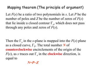
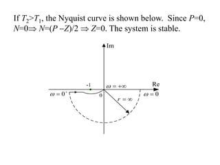
16. Nyquist contour
r 
0
S

s
jw
s-plane
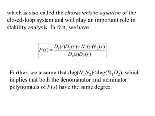
It is clear that when s traverses the semicircle of infinite
radius, F(s) remains a constant. That is, the encirclements
of the origin of F(s) only determines by F(j ) as  varies
from  to + provided that no zeros or poles lie on the
j axis.
lim ( )
lim [1 ( ) ( )] const.
s
s
F s
G s H s


  
By assumption,

17. Example.
Consider a unity feedback system whose open-loop
transfer function is as follows
2 1
( ) ( ) 1
1 1
s
G s F s G
s s

    
 
The system is stable.
1

P 1

N
0


 N
P
Z
1
 1
F(j)
0
j

18. Further, since
( ) 1
F s G
 
compare the two curves below:
1
 1
F(j)
0
j
2
 1

GH(j)
0
j
Clearly, the encirclement of the origin in F plane is
equivalent to the encirclement of 1 point in GH
plane!

19. Example.
Consider a unity feedback system whose open-loop
transfer function is as follows
0.5
( )
1
G s
s


The system is unstable.
1

P 0

N
1


 N
P
Z
1

5
.
0

G(s)
0

20. Example.
Consider a single-loop control system, where
)
1
1
.
0
)(
1
(
100
)
(
)
(



s
s
s
H
s
G
0
,
0 
 N
P
0


 N
P
Z
The system is stable. G(s)H(s)
1

0
Determine its stability.

21. Nyquist stability criterion
A system is stable if and only if from
N = PZ
we can obtain that Z=0, where P is the number of the
open-loop poles in the right-hand half s-plane and N is the
number of the encirclements of the point (1, j0) of
G(j)H(j) in the counterclockwise direction.

22. Because the plot of G(j )H(j) and the plot of
G(j )H(j) are symmetrical with each other about the
real axis. Hence, we can modify the stability criterion as
N = (P – Z)/2,
where only the polar plot of G(j)H(j) with  varying
from 0 to + is necessary.
G(s)H(s)
0
-1
Re
Im
G(s)H(s)
0
-1
Re
Im

23. Example.
Consider a unity feedback system whose open-loop
transfer function is as follows
2
( )
1
G s
s


The system is stable.
1 ( )
2 2
(1 )
0
2
P Z
N
Z
Z

 

  
Investigate its stability by using Nyquist criterion.
Solution: Obviously, P=1 (nonminimum phase plant).
Now, drawing its Nyquist plot yields:
2
 1

G(j)
0
j

24. Example.
Consider a unity feedback system whose open-loop
transfer function is as follows
1 2 3
( ) , 0, 0
( 1)( 1)( 1)
i
K
G s T K
T s T s T s
  
  
Using Nyquist plot, determine its stability.
Solution: Obviously, P=0. Now, drawing its Nyquist
plot yields:

25. 0
Im
Re
1

   0
 
1
 
N
3
K
0
Im
Re
1

   0
 
0

P
0
Im
Re
1

   0
 
0

N
1
K 2
K

26. 4. Nyquist Criterion Based on Bode diagram
Again, we consider the open-loop transfer function with
Nyquist curve below:
1 2 3
( ) , 0, 0
( 1)( 1)( 1)
i
K
G s T K
T s T s T s
  
  
where P=0, N=1 and the
system is unstable. The key
is the point that the Nyquist
curve crosses the negative
real axis is less than 1
(abs(A)>1).
0
Im
Re
1

   0
 
1
 
N
3
K
A

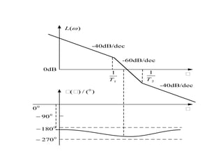
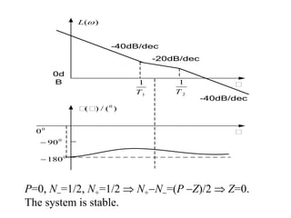
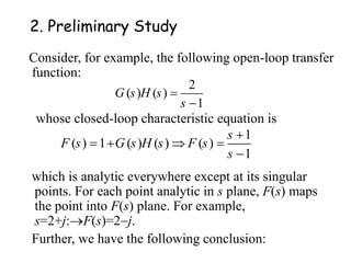
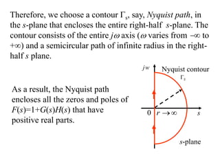
27. The Bode diagram is:
1
1
T
2
1
T 3
1
T
dB
[ 20]

[ 40]

[ 60]

20logK
w
w
0
180

0
270

c
w
0
0
G

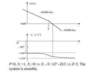
The system is unstable because the phase angle plot
crosses the1800 line in the region of 20logG(j)>0.
N=1

28. The Nyquist Theorem can be interpreted as:
Theorem: The system is stable if and only if from
N+ N = (P – Z)/2
we can obtain that Z=0.
We use N to denote the number of crosses of 1800 line
in the region of 20logG(j)>0 if each across makes
the phase angle less than 1800. Similarly, we use N+ to
denote the number of crosses of 1800 line in the region
of 20logG(j)>0 if each across makes the phase angle
larger than 1800.

29. Example. Both the Nyquist plot and Bode diagram of
an open-loop minimum phase transfer function are
shown below. Determine its stability.
)
(
GH
L lg
20


GH

1

2
 3

1
 2
 3

0
1

)
(
)
(
0
180

0 0
2 2
 
 
     
P Z Z
N N Z

30. 5. Special case when G(s)H(s) involves Poles
and Zeros on the j Axis
Consider the following open-loop transfer function:
( ) ( )
( 1)
K
G s H s
s Ts


which does not satisfy the Nyquist Theorem because s is
a singular point. Therefore, the contour s must be
modified. A way of modifying the contour near the
origin is to use a quarter-circle with an infini-tesimal
radius (>0):
j
s e q
e
 
where  varies from 00 to 900 as  varies from 0 to 0+.

31. A modified contour s :
The modified s implies
that we regard 1/s as a
stable pole.
0 0
1 1
, :0 90
j
e
s
q
q
e
-
= × - ® -
where 1/s rotates from 00 to 900 with an infinite radius
as  varies from 0 to 0+.
1
T


Radius
Re

j
s-plane
j0+
=0
Then, for the controlled plant with integral factor 1/s, we
have

32. The integral factor 1/s rotates from 00 to 900 with an
infinite radius as  varies from 0 to 0+.
1
T

Radius
r  

Radius
Re

j
j0+
=0
j

33. 
Radius
B
C
C’
Radius
r  
-1
GH-plane
u
jv
The Nyquist curve starts from real axis when =0 and
rotates 900 as =0+.
N = (P – Z)/2 Z=0, the system is stable.


j
s-plane
1
T

B’

34. L(dB)
f w
( )
135
 
90
 
10
180
 
20dB/ dec



1 1 3
T

40dB/ dec

0
 
0
 


35. Example. Let the open-loop transfer function be
2
( ) ( ) , 0, 0
( 1)
K
G s H s T K
s Ts
  

Determine its stability by using Nyquist Theorem.
Solution: When =0,
2 0
2 2
( ) ( ) , 0, 0 ;
( 1)
j
K K
G s H s e
s T s

   

q
w q
e
0
2 180
  
q
Hence, when >0+,
0 1
( ) ( ) 180 tan
G j H j T
w w w

   
When =0+,

36. 0
Im
Re
1

  
0
 

0
P 

0


P=0, N=1 N=(PZ)/2  Z=2. The system is
unstable.

37. )
(
L
-40dB/dec
-60dB/dec
0
180

0
90

0
270

T
1
0
( ) / ( )
0dB
0
0
P=0, N=1, N+=0  N+N=(P Z)/2  Z=2. The
system is unstable.

38. 6. Stability Analysis
Example. Let the open-loop transfer function be
2
1 2
2
1
( 1)
( ) ( ) , 0, 0, 0
( 1)
K T s
G s H s T T K
s T s

   

Determine its stability by using Nyquist Theorem.
Solution: When =0,
2 0
2
2 2
1
( 1)
( ) ( ) , 0, 0 ;
( 1)
j
K T s K
G s H s e
s T s


   

q
w q
e
0
0 , 2 180

   
w q
Hence, when >0+,
0 1 1
1 2
( ) ( ) 180 tan tan
G j H j T T
w w w w
 
     
When =0+

39. If T1>T2, the Nyquist curve is shown below. Since P=0,
N=1 N=(P Z)/2  Z=2. The system is unstable.



0


Re
Im

 0

-1 0

40. )
(
L
-40dB/dec
-60dB/dec
0
180

0
90

0
270

1
1
T
0
( ) / ( )
0dB
0
0
-40dB/dec
2
1
T

41. If T2>T1, the Nyquist curve is shown below. Since P=0,
N=0 N=(P Z)/2  Z=0. The system is stable.



0


Re
Im

 0

-1
0
r  

42. )
(
L
-40dB/dec
-20dB/dec
0
180

0
90

1
1
T
0
( ) / ( )
0d
B
0
0
-40dB/dec
2
1
T
P=0, N=1/2, N+=1/2  N+N=(P Z)/2  Z=0.
The system is stable.

43. Example. Consider a unity feedback system whose
open-loop transfer function is as follows
( )
( 1)


K
G s
s T s
The system is unstable.
1 ( )
2 2
(1 )
2
2
P Z
N
Z
Z

  

  
Investigate its stability by using Nyquist criterion.
Solution: Obviously, P=1 (nonminimum phase plant).
Now, drawing its Nyquist plot yields:
-1
j
  
0
 

0
 

44. 7. Conditionally Stable Systems
A conditionally stable system is stable for the value
of the open-loop gain lying between critical values, but
it is unstable if the open-loop gain is either increased or
decreased sufficiently.
0
Im
Re
1
    0
 
0
P 

45. Example. Consider a single-loop control system,
where open-loop transfer function is
)
4
2
(
)
( 2



s
s
s
K
s
G )
(s
G
Determine the range of K so that the system keeps
stable.
2
w 
n
0 0 0
( ) 90 90 180
w
     
n
G j
( 2) 1
2 4
 

K
G j
8

K
r  

46. Example. Consider a single-loop control system,
where open-loop transfer function is
1 2
3
( 1)( 1)
( )
K s s
G s
s
t t
 

Discuss its stability by using Nyquist stability
criterion.