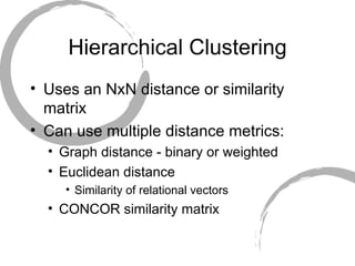
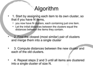
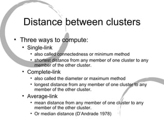
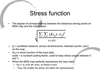
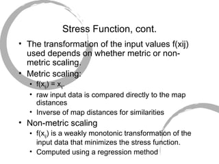
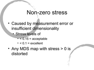
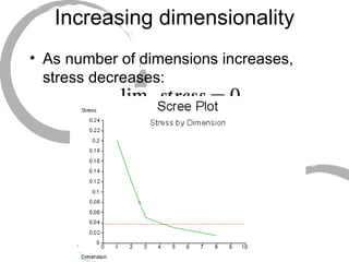
Clustering, Continued
Hierarchical Clustering Uses an NxN distance or similarity matrix Can use multiple distance metrics: Graph distance - binary or weighted Euclidean distance Similarity of relational vectors CONCOR similarity matrix
Algorithm 1. Start by assigning each item to its own cluster, so that if you have N items,  you now have N clusters, each containing just one item.  Let the initial distances between the clusters equal the distances between the items they contain. 2. Find the closest (most similar) pair of clusters and merge them into a single cluster 3. Compute distances between the new cluster and each of the old clusters. 4. Repeat steps 2 and 3 until all items are clustered into a single cluster of size N.
Distance between clusters Three ways to compute: Single-link  also called connectedness or minimum method  shortest distance from any member of one cluster to any member of the other cluster. Complete-link also called the diameter or maximum method longest distance from any member of one cluster to any member of the other cluster. Average-link mean distance from any member of one cluster to any member of the other cluster. Or median distance (D’Andrade 1978)
Preferred methods? Complete link (maximum length) clustering gives more stable results Average-link is more inclusive, has better face validity Other methods may be substituted given domain requirements
Example - US Cities Using single-link clustering BOS  NY  DC  MIA  CHI  SEA  SF  LA  DEN BOS  0  206  429  1504  963  2976  3095  2979  1949 NY  206  0  233  1308  802  2815  2934  2786  1771 DC  429  233  0  1075  671  2684  2799  2631  1616 MIA  1504  1308  1075  0  1329  3273  3053  2687  2037 CHI  963  802  671  1329  0  2013  2142  2054  996 SEA  2976  2815  2684  3273  2013  0  808  1131  1307 SF  3095  2934  2799  3053  2142  808  0  379  1235 LA  2979  2786  2631  2687  2054  1131  379  0  1059 DEN  1949  1771  1616  2037  996  1307  1235  1059  0
Example - cont. The nearest pair of cities is BOS and NY, at distance 206. These are merged into a single cluster called "BOS/NY”: BOS/NY  DC  MIA  CHI  SEA  SF  LA  DEN BOS/NY  0  223  1308  802  2815  2934  2786  1771 DC  223  0  1075  671  2684  2799  2631  1616 MIA  1308  1075  0  1329  3273  3053  2687  2037 CHI  802  671  1329  0  2013  2142  2054  996 SEA  2815  2684  3273  2013  0  808  1131  1307 SF  2934  2799  3053  2142  808  0  379  1235 LA  2786  2631  2687  2054  1131  379  0  1059 DEN  1771  1616  2037  996  1307  1235  1059  0
Example The nearest pair of objects is BOS/NY and DC, at distance 223. These are merged into a single cluster called "BOS/NY/DC".   BS/NY/DC MIA  CHI  SEA  SF  LA  DEN BS/NY/DC 0  1075  671  2684  2799  2631  1616 MIA  1075  0  1329  3273  3053  2687  2037 CHI  671  1329  0  2013  2142  2054  996 SEA  2684  3273  2013  0  808  1131  1307 SF  2799  3053  2142  808  0  379  1235 LA  2631  2687  2054  1131  379  0  1059 DEN  1616  2037  996  1307  1235  1059  0
Example BOS/NY/DC/CHI  MIA  SF/LA/SEA  DEN BOS/NY/DC/CHI  0  1075  2013  996 MIA  1075  0  2687  2037 SF/LA/SEA  2054  2687  0  1059 DEN  996  2037  1059  0 BOS/NY/DC/CHI/DEN  0  1075  1059 MIA  1075  0  2687 SF/LA/SEA  1059  2687  0 BOS/NY/DC/CHI/DEN/SF/LA/SEA  0  1075 MIA  1075  0
Example: Final Clustering In the diagram, the columns are associated with the items and the rows are associated with levels (stages) of clustering. An 'X' is placed between two columns in a given row if the corresponding items are merged at that stage in the clustering.
Comments Useful way to represent positions in social network data Discrete, well-defined algorithm Produces non-overlapping subsets Caveats Sometimes we need overlapping subsets Algorithmically, early groupings cannot be undone
Extensions Optimization-based clustering Algorithm can “add” and “remove” nodes from a cluster “ add” works similarly to hi-clus “ remove” takes a node out if it is closer to another cluster then to its own cluster Use shortest, mean or median distances “ remove” will never be invoked with max. distances Aim to improve cohesiveness of a cluster Mean distance between nodes in each cluster
Multi-Dimensional Scaling CONCOR and Hi-clustering are discrete models  Partition nodes into exhaustive non-overlapping subsets World is not so black-n-white The purpose of multidimensional scaling (MDS) is to provide a spatial representation of the pattern of similarities More similar nodes will appear closer together Finds non-intuitive equivalences in networks
Input to MDS Measure of pairwise similarity among nodes Attribute-based Euclidean distances Graph distances CONCOR similarities Output: A set of coordinates in 2D or 3D space such that Similar nodes are closer together then dissimilar nodes
Algorithm MDS finds a set of vectors in p-dimensional space such that the matrix of euclidean distances among them corresponds as closely as possible to a function of the input matrix according to a fitness  function called stress. 1. Assign points to arbitrary coordinates in p-dimensional space. 2. Compute euclidean distances among all pairs of points, to form the D’ matrix. 3. Compare the D’ matrix with the input D matrix by evaluating the stress function. The smaller the value, the greater the correspondance between the two. 4. Adjust coordinates of each point in the direction of the stress vector 5. Repeat steps 2 through 4 until stress won't get any lower
Dimensionality Normally, MDS is used in 2D space for optimal visual impact may be a very poor, highly distorted, representation of your data.  High stress value.  Increase the number of dimensions. Difficulties: High-dimensional spaces are difficult to represent visually With increasing dimensions, you must estimate an increasing number of parameters to obtain a decreasing improvement in stress.
Stress function The degree of correspondence between the distances among points on MDS map and the matrix input d ij  = euclidean distance, across all dimensions, between points i and j on the map,  f(x ij ) is some function of the input data, scale = a constant scaling factor, used to keep stress values between 0 and 1.  When the MDS map perfectly reproduces the input data,  f(x ij ) = d ij  is for all i and j, so stress is zero. Thus, the smaller the stress, the better the representation.
Stress Function, cont. The transformation of the input values f(xij) used depends on whether metric or non-metric scaling.  Metric scaling: f(x ij ) = x ij .  raw input data is compared directly to the map distances Inverse of map distances for similarities Non-metric scaling  f(x ij ) is a weakly monotonic transformation of the input data that minimizes the stress function. Computed using a regression method
Non-zero stress Caused by measurement error or insufficient dimensionality Stress levels of  < 0.15 = acceptable < 0.1 = excellent Any MDS map with stress > 0 is distorted
Increasing dimensionality As number of dimensions increases, stress decreases:
Interpretation of MDS Map Axes are meaningless We are looking at cohesiveness and proximity of clusters, not their locations Infinite number of possible permutations If stress > 0 , there is distortion Larger distances less distorted then smaller
What to look for Clusters groups of items that are closer to each other than to other items.  When really tight, highly separated clusters occur in perceptual data, it may suggest that each cluster is a domain or subdomain which should be analyzed individually.  Extract clusters and re-run MDS on them for further separation
What to look for… Dimensions  Item attributes that seem to order the items in the map along a continuum.  For example, an MDS of perceived similarities among breeds of dogs may show a distinct ordering of dogs by size.  At the same time, an independent ordering of dogs according to viciousness might be observed.  Orderings may not follow the axes or be orthogonal to each other The underlying dimensions are thought to &quot;explain&quot; the perceived similarity between items.  Implicit similarity function is a weighted sum of attributes May “discover” non-obvious continuums
High-dimensionality MDS Difficult to interpret visually, need a mathematical technique Feed MDS coordinates into another discriminator function May be easier to tease apart then original attribute vectorsm

6 Concor

  • 1.
  • 2.
    Hierarchical Clustering Usesan NxN distance or similarity matrix Can use multiple distance metrics: Graph distance - binary or weighted Euclidean distance Similarity of relational vectors CONCOR similarity matrix
  • 3.
    Algorithm 1. Startby assigning each item to its own cluster, so that if you have N items, you now have N clusters, each containing just one item. Let the initial distances between the clusters equal the distances between the items they contain. 2. Find the closest (most similar) pair of clusters and merge them into a single cluster 3. Compute distances between the new cluster and each of the old clusters. 4. Repeat steps 2 and 3 until all items are clustered into a single cluster of size N.
  • 4.
    Distance between clustersThree ways to compute: Single-link also called connectedness or minimum method shortest distance from any member of one cluster to any member of the other cluster. Complete-link also called the diameter or maximum method longest distance from any member of one cluster to any member of the other cluster. Average-link mean distance from any member of one cluster to any member of the other cluster. Or median distance (D’Andrade 1978)
  • 5.
    Preferred methods? Completelink (maximum length) clustering gives more stable results Average-link is more inclusive, has better face validity Other methods may be substituted given domain requirements
  • 6.
    Example - USCities Using single-link clustering BOS NY DC MIA CHI SEA SF LA DEN BOS 0 206 429 1504 963 2976 3095 2979 1949 NY 206 0 233 1308 802 2815 2934 2786 1771 DC 429 233 0 1075 671 2684 2799 2631 1616 MIA 1504 1308 1075 0 1329 3273 3053 2687 2037 CHI 963 802 671 1329 0 2013 2142 2054 996 SEA 2976 2815 2684 3273 2013 0 808 1131 1307 SF 3095 2934 2799 3053 2142 808 0 379 1235 LA 2979 2786 2631 2687 2054 1131 379 0 1059 DEN 1949 1771 1616 2037 996 1307 1235 1059 0
  • 7.
    Example - cont.The nearest pair of cities is BOS and NY, at distance 206. These are merged into a single cluster called &quot;BOS/NY”: BOS/NY DC MIA CHI SEA SF LA DEN BOS/NY 0 223 1308 802 2815 2934 2786 1771 DC 223 0 1075 671 2684 2799 2631 1616 MIA 1308 1075 0 1329 3273 3053 2687 2037 CHI 802 671 1329 0 2013 2142 2054 996 SEA 2815 2684 3273 2013 0 808 1131 1307 SF 2934 2799 3053 2142 808 0 379 1235 LA 2786 2631 2687 2054 1131 379 0 1059 DEN 1771 1616 2037 996 1307 1235 1059 0
  • 8.
    Example The nearestpair of objects is BOS/NY and DC, at distance 223. These are merged into a single cluster called &quot;BOS/NY/DC&quot;. BS/NY/DC MIA CHI SEA SF LA DEN BS/NY/DC 0 1075 671 2684 2799 2631 1616 MIA 1075 0 1329 3273 3053 2687 2037 CHI 671 1329 0 2013 2142 2054 996 SEA 2684 3273 2013 0 808 1131 1307 SF 2799 3053 2142 808 0 379 1235 LA 2631 2687 2054 1131 379 0 1059 DEN 1616 2037 996 1307 1235 1059 0
  • 9.
    Example BOS/NY/DC/CHI MIA SF/LA/SEA DEN BOS/NY/DC/CHI 0 1075 2013 996 MIA 1075 0 2687 2037 SF/LA/SEA 2054 2687 0 1059 DEN 996 2037 1059 0 BOS/NY/DC/CHI/DEN 0 1075 1059 MIA 1075 0 2687 SF/LA/SEA 1059 2687 0 BOS/NY/DC/CHI/DEN/SF/LA/SEA 0 1075 MIA 1075 0
  • 10.
    Example: Final ClusteringIn the diagram, the columns are associated with the items and the rows are associated with levels (stages) of clustering. An 'X' is placed between two columns in a given row if the corresponding items are merged at that stage in the clustering.
  • 11.
    Comments Useful wayto represent positions in social network data Discrete, well-defined algorithm Produces non-overlapping subsets Caveats Sometimes we need overlapping subsets Algorithmically, early groupings cannot be undone
  • 12.
    Extensions Optimization-based clusteringAlgorithm can “add” and “remove” nodes from a cluster “ add” works similarly to hi-clus “ remove” takes a node out if it is closer to another cluster then to its own cluster Use shortest, mean or median distances “ remove” will never be invoked with max. distances Aim to improve cohesiveness of a cluster Mean distance between nodes in each cluster
  • 13.
    Multi-Dimensional Scaling CONCORand Hi-clustering are discrete models Partition nodes into exhaustive non-overlapping subsets World is not so black-n-white The purpose of multidimensional scaling (MDS) is to provide a spatial representation of the pattern of similarities More similar nodes will appear closer together Finds non-intuitive equivalences in networks
  • 14.
    Input to MDSMeasure of pairwise similarity among nodes Attribute-based Euclidean distances Graph distances CONCOR similarities Output: A set of coordinates in 2D or 3D space such that Similar nodes are closer together then dissimilar nodes
  • 15.
    Algorithm MDS findsa set of vectors in p-dimensional space such that the matrix of euclidean distances among them corresponds as closely as possible to a function of the input matrix according to a fitness function called stress. 1. Assign points to arbitrary coordinates in p-dimensional space. 2. Compute euclidean distances among all pairs of points, to form the D’ matrix. 3. Compare the D’ matrix with the input D matrix by evaluating the stress function. The smaller the value, the greater the correspondance between the two. 4. Adjust coordinates of each point in the direction of the stress vector 5. Repeat steps 2 through 4 until stress won't get any lower
  • 16.
    Dimensionality Normally, MDSis used in 2D space for optimal visual impact may be a very poor, highly distorted, representation of your data. High stress value. Increase the number of dimensions. Difficulties: High-dimensional spaces are difficult to represent visually With increasing dimensions, you must estimate an increasing number of parameters to obtain a decreasing improvement in stress.
  • 17.
    Stress function Thedegree of correspondence between the distances among points on MDS map and the matrix input d ij = euclidean distance, across all dimensions, between points i and j on the map, f(x ij ) is some function of the input data, scale = a constant scaling factor, used to keep stress values between 0 and 1. When the MDS map perfectly reproduces the input data, f(x ij ) = d ij is for all i and j, so stress is zero. Thus, the smaller the stress, the better the representation.
  • 18.
    Stress Function, cont.The transformation of the input values f(xij) used depends on whether metric or non-metric scaling. Metric scaling: f(x ij ) = x ij . raw input data is compared directly to the map distances Inverse of map distances for similarities Non-metric scaling f(x ij ) is a weakly monotonic transformation of the input data that minimizes the stress function. Computed using a regression method
  • 19.
    Non-zero stress Causedby measurement error or insufficient dimensionality Stress levels of < 0.15 = acceptable < 0.1 = excellent Any MDS map with stress > 0 is distorted
  • 20.
    Increasing dimensionality Asnumber of dimensions increases, stress decreases:
  • 21.
    Interpretation of MDSMap Axes are meaningless We are looking at cohesiveness and proximity of clusters, not their locations Infinite number of possible permutations If stress > 0 , there is distortion Larger distances less distorted then smaller
  • 22.
    What to lookfor Clusters groups of items that are closer to each other than to other items. When really tight, highly separated clusters occur in perceptual data, it may suggest that each cluster is a domain or subdomain which should be analyzed individually. Extract clusters and re-run MDS on them for further separation
  • 23.
    What to lookfor… Dimensions Item attributes that seem to order the items in the map along a continuum. For example, an MDS of perceived similarities among breeds of dogs may show a distinct ordering of dogs by size. At the same time, an independent ordering of dogs according to viciousness might be observed. Orderings may not follow the axes or be orthogonal to each other The underlying dimensions are thought to &quot;explain&quot; the perceived similarity between items. Implicit similarity function is a weighted sum of attributes May “discover” non-obvious continuums
  • 24.
    High-dimensionality MDS Difficultto interpret visually, need a mathematical technique Feed MDS coordinates into another discriminator function May be easier to tease apart then original attribute vectorsm