4Probability and probability distributions.pdf

Measurements of Health and disease
Probability & probability distributions
1/3/2023 Probability & probability distributions 1
Emiru Merdassa(MSc, Assistant professor)

2
Definition
Probability: the chance that an uncertain event
will occur (always between 0 and 1)
0 ≤ P(A) ≤ 1 For any event A
Certain
Impossible
0.5
1
0
1/3/2023
Example:
• Physician may say that a patient has a 50-50 chance of
surviving a certain operation.
• 95% certain that a patient has a particular disease.
➢ Most people express probabilities in terms of
percentages.

Probability terms
• Outcomes: results of each trial
• Sample space: set of all possible outcome
• Sample points: elements of the sample space of
outcome
• Event: subset of the sample space
3
1/3/2023
(continued)

4
Important terms
• Intersection of Events – If A and B are two events in a sample
space S, then the intersection, A ∩ B, is the set of all outcomes in
S that belong to both A and B
(continued)
A B
AB
S
1/3/2023 Probability & probability distributions

5
Important terms
• Two events A and B are mutually exclusive if they cannot both
happen at the same time
• P (A ∩ B) = 0
(continued)
A B
S

6
Important terms
• Union of Events – If A and B are two events in a sample space S,
then the union, A U B, is the set of all outcomes in S that belong
to either A or B
(continued)
A B
The entire shaded area
represents
A U B
S

7
Important terms
• Events E1, E2, … Ek are Collectively Exhaustive events if E1 U E2 U
. . . U Ek = S
– i.e., the events completely cover the sample space
• The Complement of an event A is the set of all basic outcomes in
the sample space that do not belong to A. The complement is
denoted as ഥ
A
(continued)
A
S
A

8
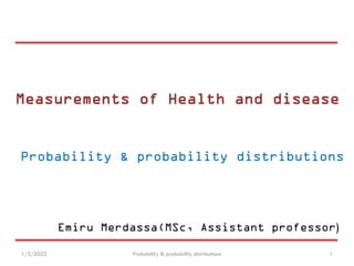
Example
Let the Sample Space be the collection of all possible
outcomes of rolling one die:
S = [1, 2, 3, 4, 5, 6]
Let A be the event “Number rolled is even”
Let B be the event “Number rolled is at least 4”
Then
A = [2, 4, 6] and B = [4, 5, 6]

9
(continued)
Example
S = [1, 2, 3, 4, 5, 6] A = [2, 4, 6] B = [4, 5, 6]
5]
3,
[1,
A =
6]
[4,
B
A =

6]
5,
4,
[2,
B
A =

S
6]
5,
4,
3,
2,
[1,
A
A =
=

Complements:
Intersections:
Unions:
[5]
B
A =

3]
2,
[1,
B =

10
Mutually exclusive:
o A and B are not mutually exclusive
• The outcomes 4 and 6 are common to both
Collectively exhaustive:
o A and B are not collectively exhaustive
• A U B does not contain 1 or 3
(continued)
Example
S = [1, 2, 3, 4, 5, 6] A = [2, 4, 6] B = [4, 5, 6]

Independent Events
• Two events A and B are independent if the probability of
the first one happening is the same no matter how the
second one turns out or
• The outcome of one event has no effect on the occurrence
or non-occurrence of the other.
P(A∩B) = P(A) x P(B) (Independent events)
P(A∩B) ≠ P(A) x P(B) (Dependent events)
Example:
O The outcomes on the first and second coin tosses are
independent
11

Continued…
Two categories of probability
1. Objective probability and
2. Subjective probability
1) Objective probability
a) Classical probability &
b) Relative frequency probability.
12

A) Classical Probability
• Is based on gambling ideas
• Example : Rolling a die
• There are 6 possible outcomes:
• Sample space = {1, 2, 3, 4, 5, 6}.
• Each is equally likely
• P(i) = 1/6, i=1,2,...,6.
→ P(1) = 1/6
→ P(2) = 1/6
…
→ P(6) = 1/6
SUM = 1
13

B) Relative Frequency Probability
• In the long run process.
• The proportion of times the event A occurs —in a large number
of trials repeated under essentially identical conditions
Definition:
• If a process is repeated a large number of times (n), and if an
event with the characteristic E occurs m times, the relative
frequency of E,
Probability of E = P(E) = m/n.
14

Example
• If you toss a coin 100 times and head comes up 40 times,
P(H) = 40/100 = 0.4.
• If we toss a coin 10,000 times and the head comes up 5562,
P(H) = 0.5562.
• Therefore, the longer the series and the longer sample size,
the closer the estimate to the true value.
15

Relative probability
• Since trials cannot be repeated an infinite number of
times, theoretical probabilities are often estimated by
empirical probabilities based on a finite amount of
data
Example:
➢ Of 158 people who attended a dinner party, 99 were ill.
➢ P (Illness) = 99/158 = 0.63 = 63%.
1/3/2023 16
(continued)

2. Subjective Probability
– Personalistic (represents one’s degree of belief in the occurrence
of an event).
– E.g., If someone says that he is 95% certain that a cure for AIDS
will be discovered within 5 years, then he means that:
– P(discovery of cure for AIDS within 5 years) = 95% = 0.95
– Although the subjective view of probability has enjoyed
increased attention over the years, it has not fully accepted by
scientists.
17

Properties of Probability
1. The numerical value of a probability always lies between 0 and 1,
inclusive(0  P(E)  1)
2. The sum of the probabilities of all mutually exclusive outcomes is
equal to 1.
P(E1) + P(E2 ) + .... + P(En ) = 1.
3. For two mutually exclusive events A and B,
P(A or B ) = P(AUB)= P(A) + P(B).
If not mutually exclusive:
P(A or B) = P(A) + P(B) - P(A and B)
1/3/2023 18

Properties of Probability
4. The complement of an event A, denoted by Ā or Ac, is the
event that A does not occur
• Consists of all the outcomes in which event A does NOT
occur: P(Ā) = P(not A) = 1 – P(A)
• Where Ā occurs only when A does not occur.
1/3/2023 19

Basic probability rules
1. Addition rule
➢ If events A and B are mutually exclusive:
P(A or B) = P(A) + P(B)
P(A and B) = 0
➢ More generally:
P(A or B) = P(A) + P(B) - P(A and B)
P(event A or event B occurs or they both occur)
20

Example
The probabilities representing years of schooling
completed by mothers of newborn infants
21
Mother’s education level Probability
≤ 8 years 0.056
9 to 11 years 0.159
12 years 0.321
13 to 15 years 0.218
≥16 years 0.230
Not reported 0.016

Continued
• What is the probability that a mother has
completed < 12 years of schooling?
P( 8 years) = 0.056 and
P(9-11 years) = 0.159
• Since these two events are mutually exclusive,
P( 8 or 9-11) = P( 8 U 9-11)
= P( 8) + P(9-11)
= 0.056+0.159
= 0.215
22

Exercise
i. Suppose two doctors, A and B, test all patients coming into a clinic for
syphilis. Let events A+ = {doctor A makes a positive diagnosis} and B+ =
{doctor B makes a positive diagnosis}.
ii. Suppose doctor A diagnoses 10% of all patients as positive, doctor B
diagnoses 17% of all patients as positive, and both doctors diagnose 8%
of all patients as positive.
➢ Suppose a patient is referred for further lab tests if either doctor A or B
makes a positive diagnosis.
 What is the probability that a patient will be referred for further lab
tests(P(Α+
∪ 𝐵+
)?
1/3/2023 23

Normal distributions
1/3/2023 24

The Normal distribution
• Normal distributions are recognized by their bell shape.
• A large percentage of the curve’s area is located near
its center and that its tails approach the horizontal axis
as asymptotes.
25

Normal distribution
1/3/2023 26
 Normal distributions are defined by:
, - < x < .
 where μ represents the mean of the distribution
and σ represents its standard deviation.
f(x) =
1
2
e
x-
2
 


−






1
2

 There are many different Normal distributions, each with
its own μ and σ, let X ~ N(μ, σ) represent a specific
member of the Normal distribution family.
 The symbol “~” is read as “distributed as.”
For example,
X ~ N(100, 15) is read as “X is a Normal random
variable with mean 100 and standard deviation 15.
1/3/2023 27

1. The mean µ tells you about location -
– Increase µ - Location shifts right
– Decrease µ – Location shifts left
– Shape is unchanged
2. The variance σ2 tells you about narrowness or flatness of the bell -
– Increase σ2 - Bell flattens. Extreme values are more likely
– Decrease σ2 - Bell narrows. Extreme values are less likely
– Location is unchanged
28

The normal distribution
Mean changes Variance changes
1/3/2023 29

30

Properties of the Normal Distribution
1. It is symmetrical about its mean, .
2. The mean, the median and mode are almost equal. It is
unimodal.
3. The total area under the curve about the x-axis is 1
square unit.
4. The curve never touches the x-axis.
5. As the value of  increases, the curve becomes more and
more flat and vice versa.
31

6. Perpendiculars of:
± 1SD contain about 68%;
±2 SD contain about 95%;
±3 SD contain about 99.7% of the area under the
curve.
7. The distribution is completely determined by the
parameters  and .
32

33

Standard Normal Distribution
It is a normal distribution that has a mean equal to 0 and a
SD equal to 1, and is denoted by N(0, 1).
The main idea is to standardize all the data that is given by
using Z-scores.
These Z-scores can then be used to find the area
(probability) under the normal curve.
34

Z - transformation
• If a random variable X~N(,) then we can transform
it to a SND with the help of Z-transformation
Z =
𝑿−

• Z represents the Z-score for a given x value
35

Continued
– Consider redefining the scale to be in terms of how many SDs
away from mean for normal distribution, μ=110 and σ = 15.
– SDs from mean using
𝒙−𝟏𝟏𝟎
𝟏𝟓
=
𝒙−

1/3/2023 36
Value x
50 65 80 95 110 125 140 155 171
-4 -3 -2 -1 0 1 2 3 4

Continued
– This process is known as standardization and gives the
position on a normal curve with μ=0 and σ=1, i.e., the
SND, Z.
– A Z-score is the number of standard deviations that a
given x value is above or below the mean.

Finding areas under the standard normal distribution curve
 The two steps are
Step 1 :
– Draw the normal distribution curve and shade the area.
Step 2:
– Find the appropriate figure in the Procedure Table and
follow the directions given.
1/3/2023 38

Procedure table
1/3/2023 39

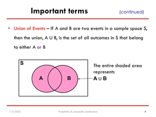
Rules in computing probabilities
P[Z = a] = 0
P[Z ≤ a] obtained directly from the Z-table
P[Z ≥ a] = 1 – P[Z ≤ a]
P[Z ≥ -a] = P[Z ≤ +a]
P[Z ≤ -a] = P[Z ≥ +a]
P[a1 ≤ Z ≤ a2] = P[Z ≤ a2] – P[Z ≤ a1]

Example 1
Find the area to the left of z = 2.06.
Solution
Step 1:
Draw the figure.
Step 2:
We are looking for the area under the standard normal distribution
to the left of z =2.06. look up the area in the table. It is 0.9803.
Hence, 98.03% of the area is less than z =2.06.
1/3/2023 41

Example 2
Find the area to the right of z = -1.19
Solution
Step 1: Draw the figure.
Step 2 : We are looking for the area to the right of z = -1.19.
Look up the area for z = -1.19. It is 0.1170. Subtract it from one.
1- 0.1170 = 0.8830. Hence, 88.30% of the area under the
standard normal distribution curve is to the right of z = -1.19.
1/3/2023 42

Continued
Example 3:
What is the probability that a z picked at random from the
population of z’s will have a value between -2.55 and +2.55 ?
 Answer : P (-2.55 < z < +2.55)
= 0.9946 – 0.0054
= 0.9892
Example 4:
What proportion of z value are between -2.47 and 1.53?
 Answer : P (-2.47 ≤ z ≤ 1.53)
= 0.9370 – 0.0068
= 0.9302

Exercises
1. Find the area between z =1.68 and z =-1.37. Ans = 0.8682
2. Find the probability for each.
a) P(0 < z <2.32) = 0.4898
b) P(z < 1.65) = 0.9505
c) P(z >1.91)= 0.0281
3. Find two z values so that 48% of the middle area is bounded
by them?
1/3/2023 44

Thank you.
1/3/2023 45

4Probability and probability distributions.pdf

Recommended

Recommended

More Related Content

Similar to 4Probability and probability distributions.pdf

Similar to 4Probability and probability distributions.pdf (20)

More from AmanuelDina

More from AmanuelDina (11)

Recently uploaded

Recently uploaded (20)

4Probability and probability distributions.pdf