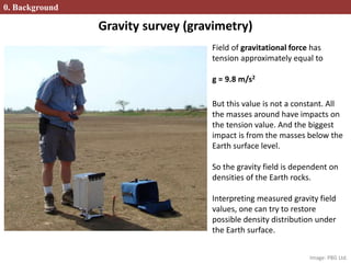
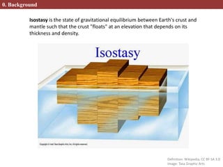
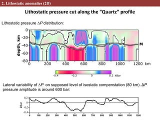
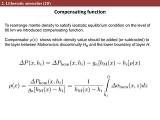
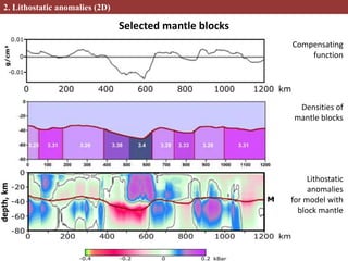
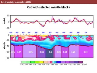
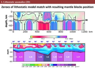
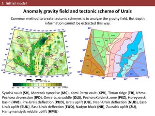
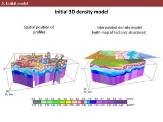
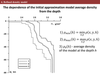
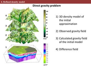
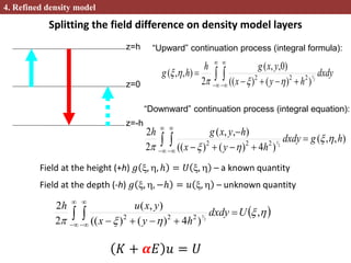
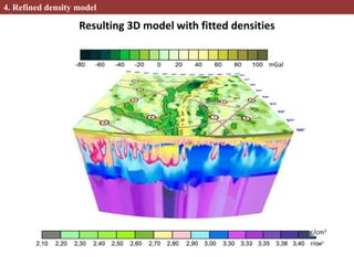
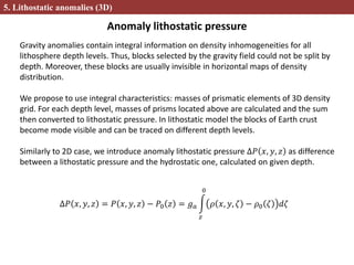
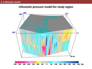
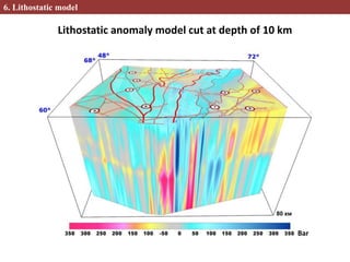
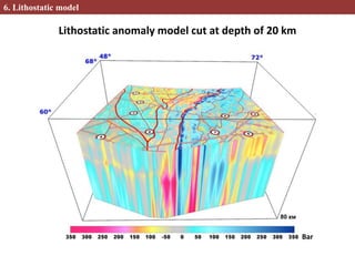
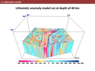
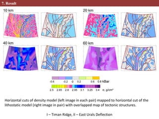
Corr. Member of RAS, Prof. Petr Martyshko1,2
Dr. Igor Ladovskii1
Denis Byzov1
Alexander Tsidaev1,2
1Bulashevich Institute of Geophysics, Yekaterinburg, Russia
2Yeltsin Ural Federal University, Yekaterinburg, Russia
2D and 3D Density Block Models Creation
Based on Isostasy Usage
REIT'2017: 1st International Workshop on Radio Electronics & Information Technologies
Gravity survey (gravimetry)
Field of gravitational force has
tension approximately equal to
g = 9.8 m/s2
But this value is not a constant. All
the masses around have impacts on
the tension value. And the biggest
impact is from the masses below the
Earth surface level.
So the gravity field is dependent on
densities of the Earth rocks.
Interpreting measured gravity field
values, one can try to restore
possible density distribution under
the Earth surface.
0. Background
Image: PBG Ltd.
0. Background
Isostasy is the state of gravitational equilibrium between Earth's crust and
mantle such that the crust "floats" at an elevation that depends on its
thickness and density.
Definition: Wikipedia, CC BY-SA 3.0
Image: Tasa Graphic Arts
Study area of Urals and neighboring regions with positions
of deep seismic sounding profiles
Profiles:
1) Agat-2
2) Globus
3) Quartz
4) V. Nildino – Kazym
5) Rubin-1
6) Syktyvkarsk
7) N. Sosva – Yalutorovsk
8) Krasnolelinsk
9) Granit – Rubin-2
10) Polar-Urals transsect
1. Initial data
mGal
Seismic-density model along the “Quartz” profile
1. Initial data
Density and velocity values are interconnected by function (Ladovskii et al., 2013).
Model with homogeneous mantle and observed (violet) and model (red) gravity fields
(model created using Mishenkina-Krylov technique)
𝑔 𝑎=9,80665 m/s2 is mean value of gravity acceleration.
∆𝑃 𝑥, 𝑧 = 𝑃 𝑥, 𝑧 − 𝑃0 𝑧 = 𝑔 𝑎
𝑧
0
𝜌 𝑥, 𝜁 − 𝜌0 𝜁 𝑑𝜁
Lithostatic pressure anomalies
The lithostatic anomaly is defined as difference between the lithostatic and
hydrostatic pressures on given depth level.
Lithostatic pressure is calculated by values of fitted densities. Hydrostatic
pressure is calculated by mean density value 𝜌0 𝑧 on every hypsometric level.
For every 𝑧 depth value the deviation ∆𝑃 𝑥, 𝑧 of lithostatic pressure 𝑃 𝑥, 𝑧
from its mean (hydrostatic) value 𝑃0 𝑧 is calculated.
2. Lithostatic anomalies (2D)
Lithostatic pressure cut along the “Quartz” profile
2. Lithostatic anomalies (2D)
Lateral variability of ∆P on supposed level of isostatic compenstation (80 km). ΔР
pressure amplitude is around 600 bar:
Lithostatic pressure ∆P distribution:
kBar
Compensating function
2. Lithostatic anomalies (2D)
To rearrange mantle density to satisfy isostatic equilibrium condition on the level of
80 km we introduced compensating function.
Compensator 𝜌 𝑥 shows which density value should be added (or subtracted) to
the layer between Mohorovicic discontinuity HM and the lower boundary of layer H.
Selected mantle blocks
2. Lithostatic anomalies (2D)
Densities of
mantle blocks
Lithostatic
anomalies
for model with
block mantle
Compensating
function
Cut with selected mantle blocks
2. Lithostatic anomalies (2D)
Zeroes of lithostatic model match with resulting mantle blocks position
2. Lithostatic anomalies (2D)
3D case
3. Initial model
Anomaly gravity field and tectonic scheme of Urals
3. Initial model
Sysolsk vault (SV), Mezensk syneclise (MC), Komi-Perm vault (KPV), Timan ridge (TR), Izhma-
Pechora depression (IPD), Omra-Luza saddle (OLS), PechoraKolvinsk zone (PKZ), Horeyversk
basin (HVB), Pre-Urals deflection (PUD), Urals uplift (UU), Near-Urals deflection (NUD), East-
Urals uplift (EUU), East-Urals deflection (EUD), Nadym block (NB), Zauralsk uplift (ZU),
Hantymansiysk middle uplift (HMU)
mGal
Common method to create tectonic schemes is to analyze the gravity field. But depth
information cannot be extracted this way.
Initial 3D density model
Interpolated density model
(with map of tectonic structures)
Spatial position of
profiles
3. Initial model
The dependence of the initial approximation model average density
from the depth
g/cm3
km
1) 𝜌 𝑚𝑖𝑛 ℎ = min
𝑥,𝑦
𝜌 𝑥, 𝑦, ℎ
2) 𝜌 𝑚𝑎𝑥 ℎ = max
𝑥,𝑦
𝜌 𝑥, 𝑦, ℎ
3) 𝜌0 ℎ - average density
of the model at the depth h
4. Refined density model
Direct gravity problem
mGal
1
1) 3D density model of
the initial
approximation
2) Observed gravity field
3) Calculated gravity field
of the initial model
4) Difference field
g/cm³
2
3
4
4. Refined density model
“Upward” continuation process (integral formula):
dxdy
hyx
yxgh
hg  



 
 2
3
))()((
)0,,(
2
),,( 222


z=0
z=-h
z=h
Splitting the field difference on density model layers
),,(
)4)()((
),,(
2
2
2
3222
hgdxdy
hyx
hyxgh





 




Field at the height (+h) 𝑔 , , ℎ = 𝑈 ,  – a known quantity
Field at the depth (-h) 𝑔 , , −ℎ = 𝑢 ,  – unknown quantity
 

,
)4)()((
),(
2
2
2
3222
Udxdy
hyx
yxuh


 




𝐾 + 𝜶𝐸 𝑢 = 𝑈
“Downward” continuation process (integral equation):
4. Refined density model
Transformation of the field difference on heights with step 1 km
∆𝑔, mGal
40 km
80 km
0 km
Field of layer below H = 00 km
g[-72; 101] mGal
4. Refined density model
Transformation of the field difference on heights with step 1 km
∆𝑔, mGal
Field of layer below H = 05 km
g[-24; 44] mGal
40 km
80 km
0 km
4. Refined density model
Transformation of the field difference on heights with step 1 km
∆𝑔, mGal
Field of layer below H = 20 km
g[-43; 51] mGal
40 km
80 km
0 km
4. Refined density model
Transformation of the field difference on heights with step 1 km
∆𝑔, mGal
Field of layer below H = 40 km
g[-15; 15] mGal
40 km
80 km
0 km
4. Refined density model
Transformation of the field difference on heights with step 1 km
∆𝑔, mGal
Field of layer below H = 80 km
g[-8; 7] mGal
40 km
80 km
0 km
4. Refined density model
mGal
g/cm3
Resulting 3D model with fitted densities
Anomaly lithostatic pressure
5. Lithostatic anomalies (3D)
Gravity anomalies contain integral information on density inhomogeneities for all
lithosphere depth levels. Thus, blocks selected by the gravity field could not be split by
depth. Moreover, these blocks are usually invisible in horizontal maps of density
distribution.
We propose to use integral characteristics: masses of prismatic elements of 3D density
grid. For each depth level, masses of prisms located above are calculated and the sum
then converted to lithostatic pressure. In lithostatic model the blocks of Earth crust
become mode visible and can be traced on different depth levels.
Similarly to 2D case, we introduce anomaly lithostatic pressure ∆𝑃 𝑥, 𝑦, 𝑧 as difference
between a lithostatic pressure and the hydrostatic one, calculated on given depth.
∆𝑃 𝑥, 𝑦, 𝑧 = 𝑃 𝑥, 𝑦, 𝑧 − 𝑃0 𝑧 = 𝑔 𝑎
𝑧
0
𝜌 𝑥, 𝑦, 𝜁 − 𝜌0 𝜁 𝑑𝜁
6. Lithostatic model
Bar
Lithostatic pressure model for study region
Lithostatic anomaly model cut at depth of 10 km
6. Lithostatic model
Bar
6. Lithostatic model
Lithostatic anomaly model cut at depth of 20 km
Bar
6. Lithostatic model
Lithostatic anomaly model cut at depth of 40 km
Bar
Horizontal cuts of density model (left image in each pair) mapped to horizontal cut of the
lithostatic model (right image in pair) with overlapped map of tectonic structures.
I – Timan Ridge, II – East Urals Deflection
7. Result
8. Conclusion
• Matching of 3D lithostatic model with density model allowed us to select large deep
inhomogeneities in the upper lithosphere.
• Distribution of lithostatic pressure on horizontal cuts qualitatively matches the map of
tectonic structures, which was created by potential fields.
• Block structures positions coincides with the deep fault boundaries of collision
structures: East boundary of Timan ridge, Pechora-Kolvinsk zone, Near-Urals Deflection,
Western edge of Tagil deflection (Main Urals Fault) and zone of East-Urals uplift and
East-Urals deflection conjunction.
• Such a separation of continual density model to separate layers and blocks of different
organization level allows one to build seismic-gravity model of layers and blocks for the
Earth crust in a study region.
Conclusion
9. Literature
Ladovsky, I.V., Martyshko, P.S., Druzhinin, V.S., Byzov, D.D., Tsidaev, A.G., Kolmogorova V.V.: Methods
and results of crust and upper mantle volume density modeling for deep structure of the Middle Urals
region.
Ural Geophysical Messenger. 2(22), 31-45 (2013) [in Russian]
Martyshko, P.S., Ladovskii, I.V., Byzov, D.D.: Solution of the Gravimetric Inverse
Problem Using Multidimensional Grids.
Doklady Earth Sciences. 450, Part 2, 666-671 (2013)
Martyshko, P.S., Ladovskiy, I.V., Byzov, D.D.: Stable methods of interpretation of gravimetric data.
Doklady Earth Sciences. 471, Issue 2, 1319{1322 (2016)
Martyshko, P.S., Ladovskiy, I.V., Fedorova, N.V., Byzov, D.D., Tsidaev, A.G.: Theory and methods of
complex interpretation of geophysical data. UrO RAN, Ekaterinburg (2016) [in Russian]
http://igeoph.net/book.pdf
Thank you for your attention
10. Questions?

2D and 3D Density Block Models Creation Based on Isostasy Usage

  • 1.
    Corr. Member ofRAS, Prof. Petr Martyshko1,2 Dr. Igor Ladovskii1 Denis Byzov1 Alexander Tsidaev1,2 1Bulashevich Institute of Geophysics, Yekaterinburg, Russia 2Yeltsin Ural Federal University, Yekaterinburg, Russia 2D and 3D Density Block Models Creation Based on Isostasy Usage REIT'2017: 1st International Workshop on Radio Electronics & Information Technologies
  • 2.
    Gravity survey (gravimetry) Fieldof gravitational force has tension approximately equal to g = 9.8 m/s2 But this value is not a constant. All the masses around have impacts on the tension value. And the biggest impact is from the masses below the Earth surface level. So the gravity field is dependent on densities of the Earth rocks. Interpreting measured gravity field values, one can try to restore possible density distribution under the Earth surface. 0. Background Image: PBG Ltd.
  • 3.
    0. Background Isostasy isthe state of gravitational equilibrium between Earth's crust and mantle such that the crust "floats" at an elevation that depends on its thickness and density. Definition: Wikipedia, CC BY-SA 3.0 Image: Tasa Graphic Arts
  • 4.
    Study area ofUrals and neighboring regions with positions of deep seismic sounding profiles Profiles: 1) Agat-2 2) Globus 3) Quartz 4) V. Nildino – Kazym 5) Rubin-1 6) Syktyvkarsk 7) N. Sosva – Yalutorovsk 8) Krasnolelinsk 9) Granit – Rubin-2 10) Polar-Urals transsect 1. Initial data mGal
  • 5.
    Seismic-density model alongthe “Quartz” profile 1. Initial data Density and velocity values are interconnected by function (Ladovskii et al., 2013). Model with homogeneous mantle and observed (violet) and model (red) gravity fields (model created using Mishenkina-Krylov technique)
  • 6.
    𝑔 𝑎=9,80665 m/s2is mean value of gravity acceleration. ∆𝑃 𝑥, 𝑧 = 𝑃 𝑥, 𝑧 − 𝑃0 𝑧 = 𝑔 𝑎 𝑧 0 𝜌 𝑥, 𝜁 − 𝜌0 𝜁 𝑑𝜁 Lithostatic pressure anomalies The lithostatic anomaly is defined as difference between the lithostatic and hydrostatic pressures on given depth level. Lithostatic pressure is calculated by values of fitted densities. Hydrostatic pressure is calculated by mean density value 𝜌0 𝑧 on every hypsometric level. For every 𝑧 depth value the deviation ∆𝑃 𝑥, 𝑧 of lithostatic pressure 𝑃 𝑥, 𝑧 from its mean (hydrostatic) value 𝑃0 𝑧 is calculated. 2. Lithostatic anomalies (2D)
  • 7.
    Lithostatic pressure cutalong the “Quartz” profile 2. Lithostatic anomalies (2D) Lateral variability of ∆P on supposed level of isostatic compenstation (80 km). ΔР pressure amplitude is around 600 bar: Lithostatic pressure ∆P distribution: kBar
  • 8.
    Compensating function 2. Lithostaticanomalies (2D) To rearrange mantle density to satisfy isostatic equilibrium condition on the level of 80 km we introduced compensating function. Compensator 𝜌 𝑥 shows which density value should be added (or subtracted) to the layer between Mohorovicic discontinuity HM and the lower boundary of layer H.
  • 9.
    Selected mantle blocks 2.Lithostatic anomalies (2D) Densities of mantle blocks Lithostatic anomalies for model with block mantle Compensating function
  • 10.
    Cut with selectedmantle blocks 2. Lithostatic anomalies (2D)
  • 11.
    Zeroes of lithostaticmodel match with resulting mantle blocks position 2. Lithostatic anomalies (2D)
  • 12.
  • 13.
    Anomaly gravity fieldand tectonic scheme of Urals 3. Initial model Sysolsk vault (SV), Mezensk syneclise (MC), Komi-Perm vault (KPV), Timan ridge (TR), Izhma- Pechora depression (IPD), Omra-Luza saddle (OLS), PechoraKolvinsk zone (PKZ), Horeyversk basin (HVB), Pre-Urals deflection (PUD), Urals uplift (UU), Near-Urals deflection (NUD), East- Urals uplift (EUU), East-Urals deflection (EUD), Nadym block (NB), Zauralsk uplift (ZU), Hantymansiysk middle uplift (HMU) mGal Common method to create tectonic schemes is to analyze the gravity field. But depth information cannot be extracted this way.
  • 14.
    Initial 3D densitymodel Interpolated density model (with map of tectonic structures) Spatial position of profiles 3. Initial model
  • 15.
    The dependence ofthe initial approximation model average density from the depth g/cm3 km 1) 𝜌 𝑚𝑖𝑛 ℎ = min 𝑥,𝑦 𝜌 𝑥, 𝑦, ℎ 2) 𝜌 𝑚𝑎𝑥 ℎ = max 𝑥,𝑦 𝜌 𝑥, 𝑦, ℎ 3) 𝜌0 ℎ - average density of the model at the depth h 4. Refined density model
  • 16.
    Direct gravity problem mGal 1 1)3D density model of the initial approximation 2) Observed gravity field 3) Calculated gravity field of the initial model 4) Difference field g/cm³ 2 3 4 4. Refined density model
  • 17.
    “Upward” continuation process(integral formula): dxdy hyx yxgh hg         2 3 ))()(( )0,,( 2 ),,( 222   z=0 z=-h z=h Splitting the field difference on density model layers ),,( )4)()(( ),,( 2 2 2 3222 hgdxdy hyx hyxgh            Field at the height (+h) 𝑔 , , ℎ = 𝑈 ,  – a known quantity Field at the depth (-h) 𝑔 , , −ℎ = 𝑢 ,  – unknown quantity    , )4)()(( ),( 2 2 2 3222 Udxdy hyx yxuh         𝐾 + 𝜶𝐸 𝑢 = 𝑈 “Downward” continuation process (integral equation): 4. Refined density model
  • 18.
    Transformation of thefield difference on heights with step 1 km ∆𝑔, mGal 40 km 80 km 0 km Field of layer below H = 00 km g[-72; 101] mGal 4. Refined density model
  • 19.
    Transformation of thefield difference on heights with step 1 km ∆𝑔, mGal Field of layer below H = 05 km g[-24; 44] mGal 40 km 80 km 0 km 4. Refined density model
  • 20.
    Transformation of thefield difference on heights with step 1 km ∆𝑔, mGal Field of layer below H = 20 km g[-43; 51] mGal 40 km 80 km 0 km 4. Refined density model
  • 21.
    Transformation of thefield difference on heights with step 1 km ∆𝑔, mGal Field of layer below H = 40 km g[-15; 15] mGal 40 km 80 km 0 km 4. Refined density model
  • 22.
    Transformation of thefield difference on heights with step 1 km ∆𝑔, mGal Field of layer below H = 80 km g[-8; 7] mGal 40 km 80 km 0 km 4. Refined density model
  • 23.
    4. Refined densitymodel mGal g/cm3 Resulting 3D model with fitted densities
  • 24.
    Anomaly lithostatic pressure 5.Lithostatic anomalies (3D) Gravity anomalies contain integral information on density inhomogeneities for all lithosphere depth levels. Thus, blocks selected by the gravity field could not be split by depth. Moreover, these blocks are usually invisible in horizontal maps of density distribution. We propose to use integral characteristics: masses of prismatic elements of 3D density grid. For each depth level, masses of prisms located above are calculated and the sum then converted to lithostatic pressure. In lithostatic model the blocks of Earth crust become mode visible and can be traced on different depth levels. Similarly to 2D case, we introduce anomaly lithostatic pressure ∆𝑃 𝑥, 𝑦, 𝑧 as difference between a lithostatic pressure and the hydrostatic one, calculated on given depth. ∆𝑃 𝑥, 𝑦, 𝑧 = 𝑃 𝑥, 𝑦, 𝑧 − 𝑃0 𝑧 = 𝑔 𝑎 𝑧 0 𝜌 𝑥, 𝑦, 𝜁 − 𝜌0 𝜁 𝑑𝜁
  • 25.
    6. Lithostatic model Bar Lithostaticpressure model for study region
  • 26.
    Lithostatic anomaly modelcut at depth of 10 km 6. Lithostatic model Bar
  • 27.
    6. Lithostatic model Lithostaticanomaly model cut at depth of 20 km Bar
  • 28.
    6. Lithostatic model Lithostaticanomaly model cut at depth of 40 km Bar
  • 29.
    Horizontal cuts ofdensity model (left image in each pair) mapped to horizontal cut of the lithostatic model (right image in pair) with overlapped map of tectonic structures. I – Timan Ridge, II – East Urals Deflection 7. Result
  • 30.
    8. Conclusion • Matchingof 3D lithostatic model with density model allowed us to select large deep inhomogeneities in the upper lithosphere. • Distribution of lithostatic pressure on horizontal cuts qualitatively matches the map of tectonic structures, which was created by potential fields. • Block structures positions coincides with the deep fault boundaries of collision structures: East boundary of Timan ridge, Pechora-Kolvinsk zone, Near-Urals Deflection, Western edge of Tagil deflection (Main Urals Fault) and zone of East-Urals uplift and East-Urals deflection conjunction. • Such a separation of continual density model to separate layers and blocks of different organization level allows one to build seismic-gravity model of layers and blocks for the Earth crust in a study region. Conclusion
  • 31.
    9. Literature Ladovsky, I.V.,Martyshko, P.S., Druzhinin, V.S., Byzov, D.D., Tsidaev, A.G., Kolmogorova V.V.: Methods and results of crust and upper mantle volume density modeling for deep structure of the Middle Urals region. Ural Geophysical Messenger. 2(22), 31-45 (2013) [in Russian] Martyshko, P.S., Ladovskii, I.V., Byzov, D.D.: Solution of the Gravimetric Inverse Problem Using Multidimensional Grids. Doklady Earth Sciences. 450, Part 2, 666-671 (2013) Martyshko, P.S., Ladovskiy, I.V., Byzov, D.D.: Stable methods of interpretation of gravimetric data. Doklady Earth Sciences. 471, Issue 2, 1319{1322 (2016) Martyshko, P.S., Ladovskiy, I.V., Fedorova, N.V., Byzov, D.D., Tsidaev, A.G.: Theory and methods of complex interpretation of geophysical data. UrO RAN, Ekaterinburg (2016) [in Russian] http://igeoph.net/book.pdf
  • 32.
    Thank you foryour attention 10. Questions?

Editor's Notes

  • #8 То же самое сделаем в 3D
  • #12 Блоки видны и в неуравновешенной модели
  • #15 Профили уже с блочной мантией, но после интерполяции блоки перестают быть четкими блоками
  • #24 Модель, уже удовлетворяющая наблюденному полю