Optimal Scanning of Gaussian
and Fractal Brownian Images
with an Estimation of
Correlation Dimension
A.Yu. Parshin, PhD,
Prof. Yu.N. Parshin, Doctor of Technical Sciences
Ryazan State Radio Engineering University, Ryazan, Russia
parshin.y.n@rsreu.ru
Already known scanning methods
Static scanning methods
◦ Usual scanning methods – vertical, horizontal, diagonal.
◦ Space-filling curves – Peano-Hilbert curves.
Adaptive scanning methods
◦ Choosing scanning method for every image.
◦ Calculation of information parameter and considering it as criterion of scanning direction.
Calculation of correlation dimension
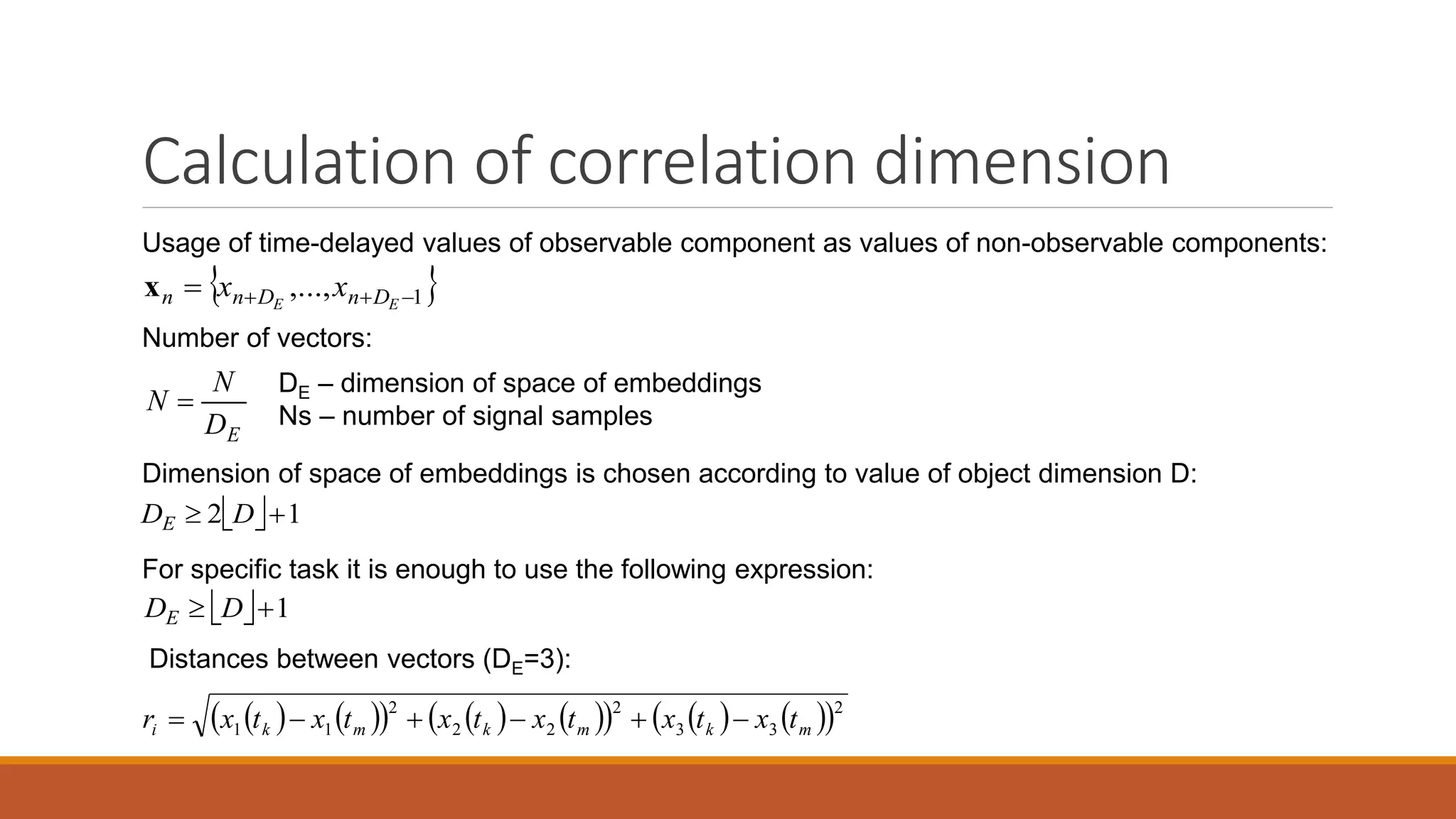
Usage of time-delayed values of observable component as values of non-observable components:
Distances between vectors (DE=3):
              2
33
2
22
2
11 mkmkmki txtxtxtxtxtxr 
Number of vectors:
ED
N
N 
DE – dimension of space of embeddings
Ns – number of signal samples
 1,...,  EE DnDnn xxx
  12  DDE
  1 DDE
Dimension of space of embeddings is chosen according to value of object dimension D:
For specific task it is enough to use the following expression:
Calculation of correlation dimension
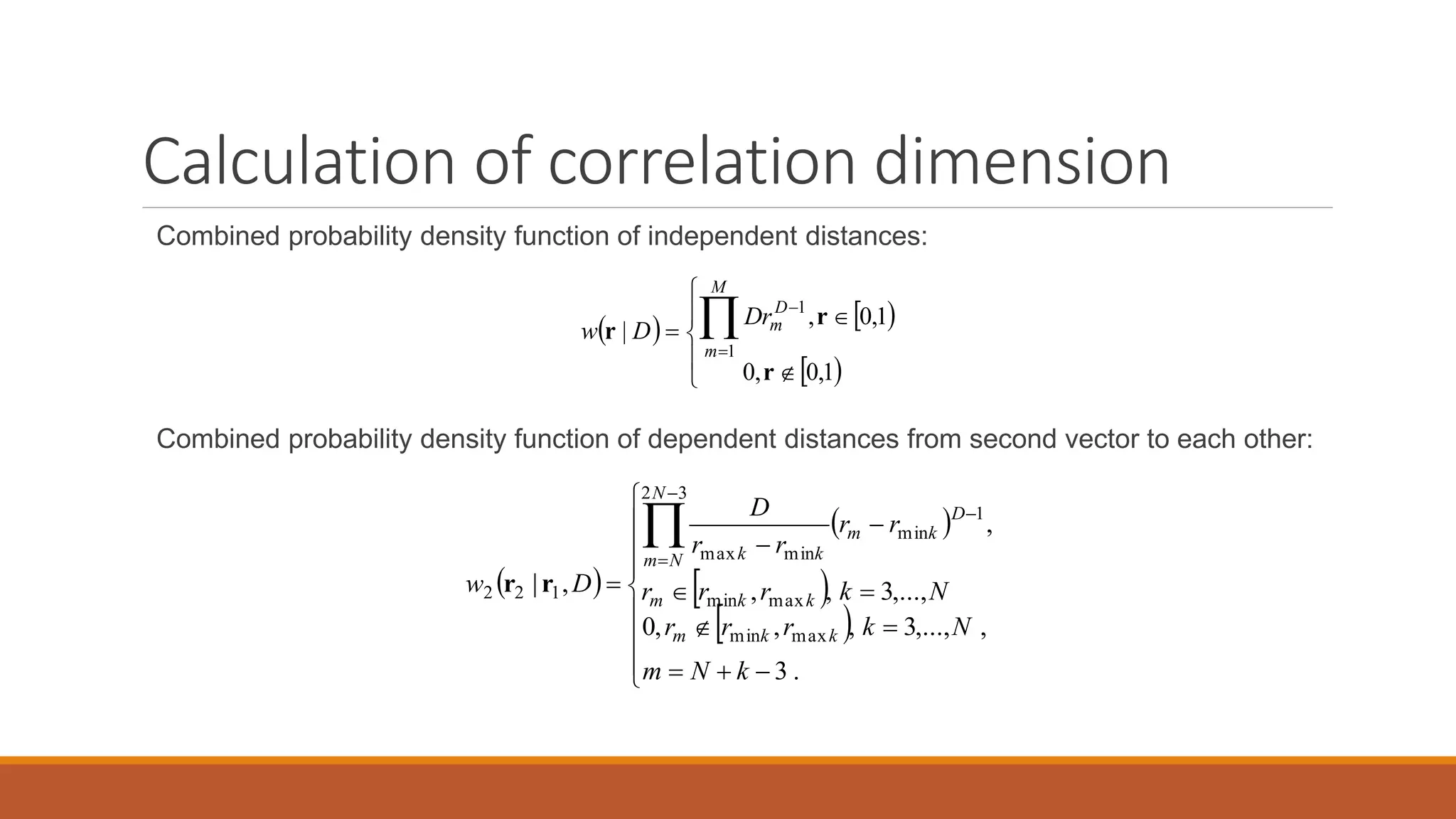
Combined probability density function of independent distances:
Combined probability density function of dependent distances from second vector to each other:
   
 










1,0,0
1,0,
|
1
1
r
r
r
D
m
M
m
rD
Dw
 
 
 
 



















.3
,,...,3,,,0
,...,3,,
,
,|
maxmin
maxmin
1
min
32
minmax
122
kNm
Nkrrr
Nkrrr
rr
rr
D
Dw
kkm
kkm
D
km
N
Nm kk
rr
Calculation of correlation dimension
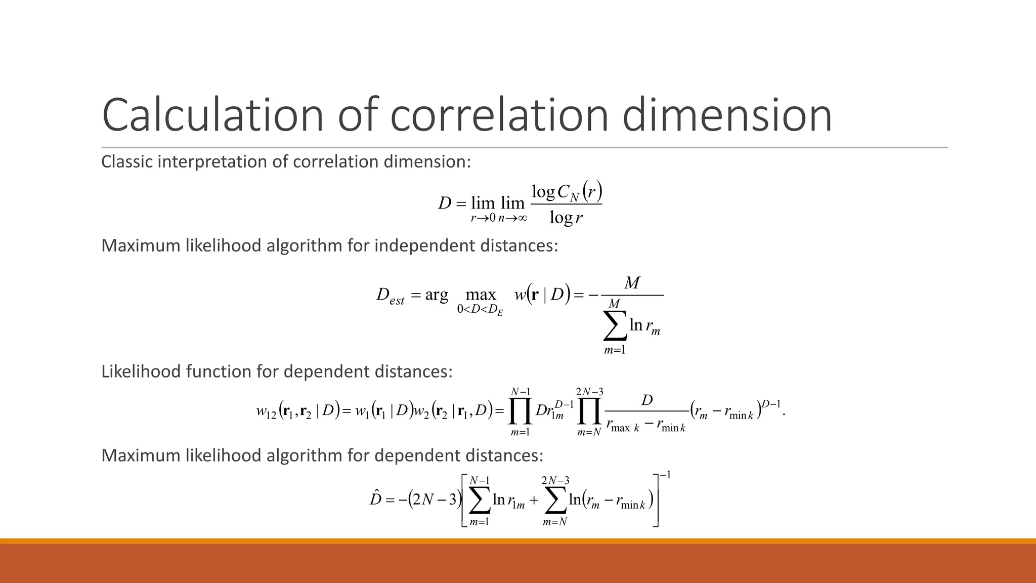
Classic interpretation of correlation dimension:
Maximum likelihood algorithm for independent distances:
Likelihood function for dependent distances:
Maximum likelihood algorithm for dependent distances:
 


 M
m
m
DD
est
r
M
DwD
E
1
0
ln
|maxarg r
        .,|||, 1
min
32
minmax
1
1
1
1
122112112








  D
km
N
Nm kk
D
m
N
m
rr
rr
D
rDDwDwDw rrrrr
   
1
32
min
1
1
1 lnln32ˆ




 







 
N
Nm
km
N
m
m rrrND
 
r
rC
D N
nr log
log
limlim
0 

Correlation function of fractal Brownian
surface
The correlation of the pixels series is specified as follows:
Let us define a fractal Brownian surface as an assembly of the random values X(i,j) given on the
2D coordinate axis. A probability measure of the random value increments:
the correlation coefficient of increments equals:
        2211221121 ,,,,,, kkkkkkkks jijiRjipjipkkR  M
       jiXjjiiXjiXjiXX ,,,, 1122 
 
    1
1
,,,
2
2
1
2
1
2
12
2
12
2211












H
ji
jjii
jijir
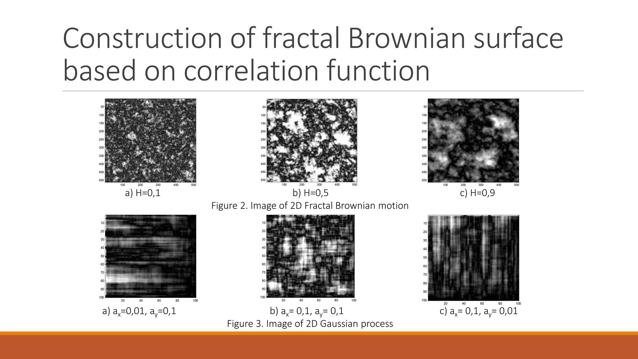
Construction of fractal Brownian surface
based on correlation function
100 200 300 400 500
50
100
150
200
250
300
350
400
450
500
100 200 300 400 500
50
100
150
200
250
300
350
400
450
500
100 200 300 400 500
50
100
150
200
250
300
350
400
450
500
20 40 60 80 100
10
20
30
40
50
60
70
80
90
100
20 40 60 80 100
10
20
30
40
50
60
70
80
90
100
20 40 60 80 100
10
20
30
40
50
60
70
80
90
100
a) H=0,1 b) H=0,5 c) H=0,9
Figure 2. Image of 2D Fractal Brownian motion
a) ax=0,01, ay=0,1 b) ax= 0,1, ay= 0,1 c) ax= 0,1, ay= 0,01
Figure 3. Image of 2D Gaussian process
Proposed scanning methods
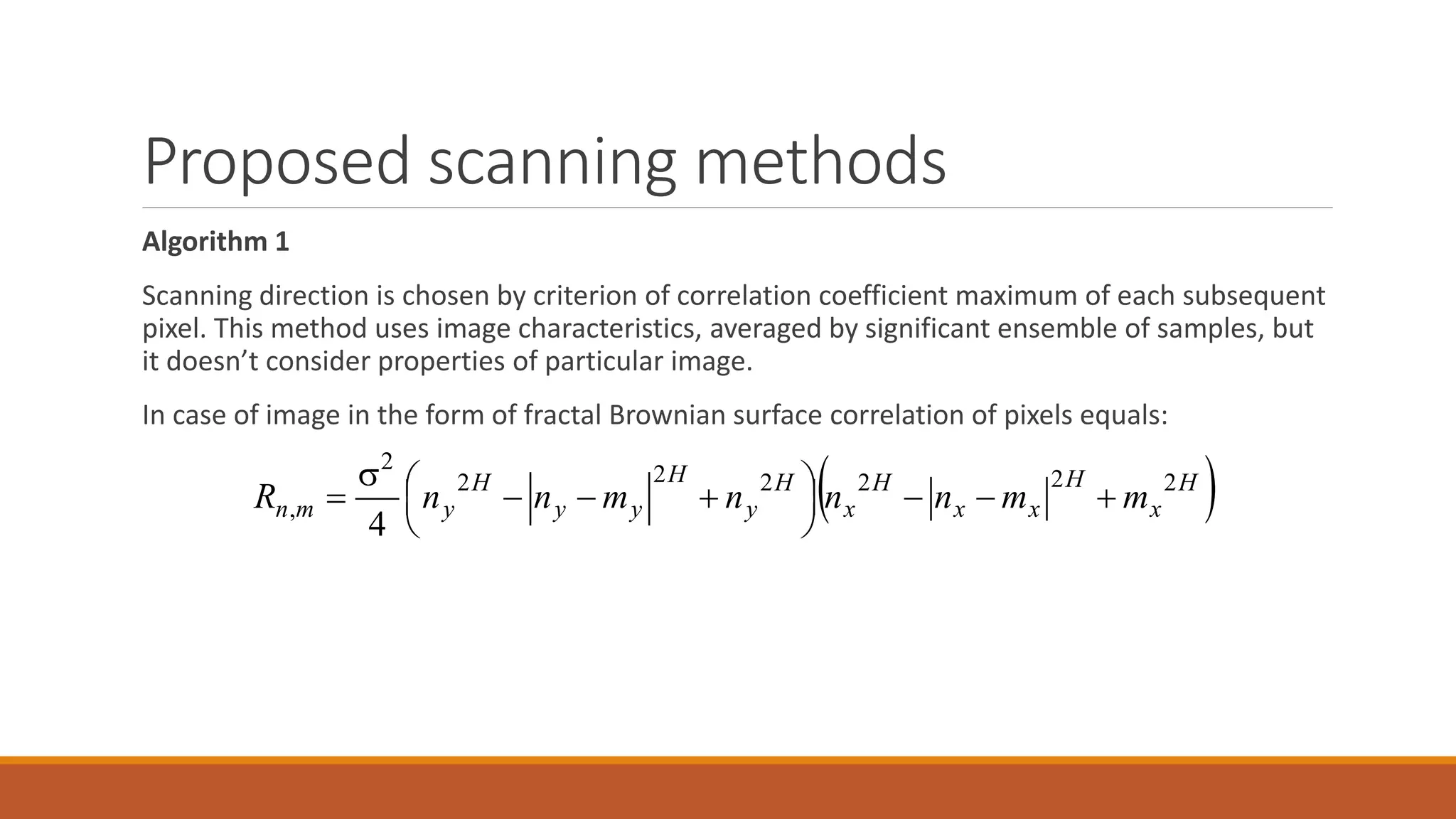
Algorithm 1
Scanning direction is chosen by criterion of correlation coefficient maximum of each subsequent
pixel. This method uses image characteristics, averaged by significant ensemble of samples, but
it doesn’t consider properties of particular image.
In case of image in the form of fractal Brownian surface correlation of pixels equals:
 H
x
H
xx
H
x
H
y
H
yy
H
ymn mmnnnmnnR 222222
2
,
4





 


Proposed scanning methods
Algorithm 2
Scanning direction is chosen by criterion of scalar product maximum of previous vector X and
following vector Y.
Steps of this algorithm:
◦ First vector consists of M image pixels from first line of current frame;
◦ One of Q predefined directions from last pixel to end of next vector is considered;
◦ standard scalar product is evaluated for pair of vectors previous X and each of Q considered directions Y
as follows:
◦ maximum value of scalar product defines a pair of vectors and thereby the direction of scan trajectory;
◦ scan trajectory moves to new pixel, which is last for chosen vector;
◦ the algorithm is repeated until majority pixels are covered.
 
YX
YX
YX


,
,R
Optimal scanning trajectories
0 10 20 30 40 50 60 70
0
10
20
30
40
50
60
70
0 10 20 30 40 50 60 70
0
10
20
30
40
50
60
70
10 20 30 40 50 60
10
20
30
40
50
60
10 20 30 40 50 60
10
20
30
40
50
60
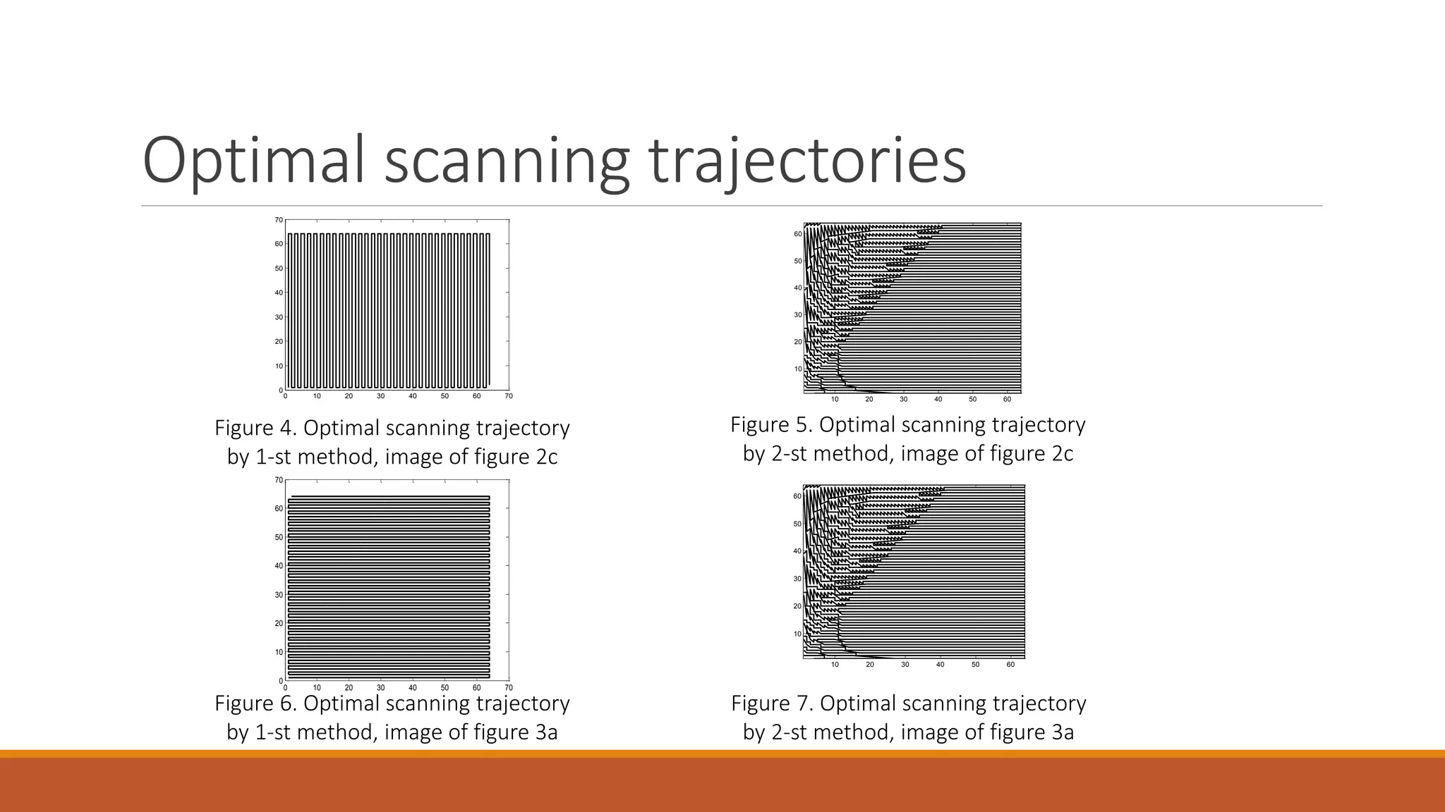
Figure 4. Optimal scanning trajectory
by 1-st method, image of figure 2c
Figure 5. Optimal scanning trajectory
by 2-st method, image of figure 2c
Figure 6. Optimal scanning trajectory
by 1-st method, image of figure 3a
Figure 7. Optimal scanning trajectory
by 2-st method, image of figure 3a
Correlation dimension estimation
0 0.2 0.4 0.6 0.8 1
0
2
4
6
8
10De
H
0 0.2 0.4 0.6 0.8 1
0
2
4
6
8
10
De
H
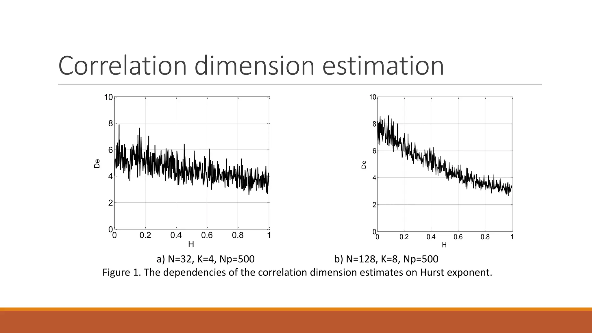
a) N=32, K=4, Np=500 b) N=128, K=8, Np=500
Figure 1. The dependencies of the correlation dimension estimates on Hurst exponent.
Conclusion
◦ Appliance of maximum likelihood algorithm demands provision of maximum
correlations between image pixels in one-dimension sequence.
◦ Scanning by maximum correlation coefficient criterion provides bigger
difference between values of correlation dimension estimates and therefore
simplifies solution of object detection problem.
Thanks for Your attention!

Optimal Scanning of Gaussian and Fractal Brownian Images with an Estimation of Correlation Dimension

  • 1.
    Optimal Scanning ofGaussian and Fractal Brownian Images with an Estimation of Correlation Dimension A.Yu. Parshin, PhD, Prof. Yu.N. Parshin, Doctor of Technical Sciences Ryazan State Radio Engineering University, Ryazan, Russia parshin.y.n@rsreu.ru
  • 2.
    Already known scanningmethods Static scanning methods ◦ Usual scanning methods – vertical, horizontal, diagonal. ◦ Space-filling curves – Peano-Hilbert curves. Adaptive scanning methods ◦ Choosing scanning method for every image. ◦ Calculation of information parameter and considering it as criterion of scanning direction.
  • 3.
    Calculation of correlationdimension Usage of time-delayed values of observable component as values of non-observable components: Distances between vectors (DE=3):               2 33 2 22 2 11 mkmkmki txtxtxtxtxtxr  Number of vectors: ED N N  DE – dimension of space of embeddings Ns – number of signal samples  1,...,  EE DnDnn xxx   12  DDE   1 DDE Dimension of space of embeddings is chosen according to value of object dimension D: For specific task it is enough to use the following expression:
  • 4.
    Calculation of correlationdimension Combined probability density function of independent distances: Combined probability density function of dependent distances from second vector to each other:                 1,0,0 1,0, | 1 1 r r r D m M m rD Dw                            .3 ,,...,3,,,0 ,...,3,, , ,| maxmin maxmin 1 min 32 minmax 122 kNm Nkrrr Nkrrr rr rr D Dw kkm kkm D km N Nm kk rr
  • 5.
    Calculation of correlationdimension Classic interpretation of correlation dimension: Maximum likelihood algorithm for independent distances: Likelihood function for dependent distances: Maximum likelihood algorithm for dependent distances:      M m m DD est r M DwD E 1 0 ln |maxarg r         .,|||, 1 min 32 minmax 1 1 1 1 122112112           D km N Nm kk D m N m rr rr D rDDwDwDw rrrrr     1 32 min 1 1 1 lnln32ˆ                N Nm km N m m rrrND   r rC D N nr log log limlim 0  
  • 6.
    Correlation function offractal Brownian surface The correlation of the pixels series is specified as follows: Let us define a fractal Brownian surface as an assembly of the random values X(i,j) given on the 2D coordinate axis. A probability measure of the random value increments: the correlation coefficient of increments equals:         2211221121 ,,,,,, kkkkkkkks jijiRjipjipkkR  M        jiXjjiiXjiXjiXX ,,,, 1122        1 1 ,,, 2 2 1 2 1 2 12 2 12 2211             H ji jjii jijir
  • 7.
    Construction of fractalBrownian surface based on correlation function 100 200 300 400 500 50 100 150 200 250 300 350 400 450 500 100 200 300 400 500 50 100 150 200 250 300 350 400 450 500 100 200 300 400 500 50 100 150 200 250 300 350 400 450 500 20 40 60 80 100 10 20 30 40 50 60 70 80 90 100 20 40 60 80 100 10 20 30 40 50 60 70 80 90 100 20 40 60 80 100 10 20 30 40 50 60 70 80 90 100 a) H=0,1 b) H=0,5 c) H=0,9 Figure 2. Image of 2D Fractal Brownian motion a) ax=0,01, ay=0,1 b) ax= 0,1, ay= 0,1 c) ax= 0,1, ay= 0,01 Figure 3. Image of 2D Gaussian process
  • 8.
    Proposed scanning methods Algorithm1 Scanning direction is chosen by criterion of correlation coefficient maximum of each subsequent pixel. This method uses image characteristics, averaged by significant ensemble of samples, but it doesn’t consider properties of particular image. In case of image in the form of fractal Brownian surface correlation of pixels equals:  H x H xx H x H y H yy H ymn mmnnnmnnR 222222 2 , 4         
  • 9.
    Proposed scanning methods Algorithm2 Scanning direction is chosen by criterion of scalar product maximum of previous vector X and following vector Y. Steps of this algorithm: ◦ First vector consists of M image pixels from first line of current frame; ◦ One of Q predefined directions from last pixel to end of next vector is considered; ◦ standard scalar product is evaluated for pair of vectors previous X and each of Q considered directions Y as follows: ◦ maximum value of scalar product defines a pair of vectors and thereby the direction of scan trajectory; ◦ scan trajectory moves to new pixel, which is last for chosen vector; ◦ the algorithm is repeated until majority pixels are covered.   YX YX YX   , ,R
  • 10.
    Optimal scanning trajectories 010 20 30 40 50 60 70 0 10 20 30 40 50 60 70 0 10 20 30 40 50 60 70 0 10 20 30 40 50 60 70 10 20 30 40 50 60 10 20 30 40 50 60 10 20 30 40 50 60 10 20 30 40 50 60 Figure 4. Optimal scanning trajectory by 1-st method, image of figure 2c Figure 5. Optimal scanning trajectory by 2-st method, image of figure 2c Figure 6. Optimal scanning trajectory by 1-st method, image of figure 3a Figure 7. Optimal scanning trajectory by 2-st method, image of figure 3a
  • 11.
    Correlation dimension estimation 00.2 0.4 0.6 0.8 1 0 2 4 6 8 10De H 0 0.2 0.4 0.6 0.8 1 0 2 4 6 8 10 De H a) N=32, K=4, Np=500 b) N=128, K=8, Np=500 Figure 1. The dependencies of the correlation dimension estimates on Hurst exponent.
  • 12.
    Conclusion ◦ Appliance ofmaximum likelihood algorithm demands provision of maximum correlations between image pixels in one-dimension sequence. ◦ Scanning by maximum correlation coefficient criterion provides bigger difference between values of correlation dimension estimates and therefore simplifies solution of object detection problem.
  • 13.
    Thanks for Yourattention!