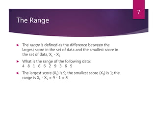
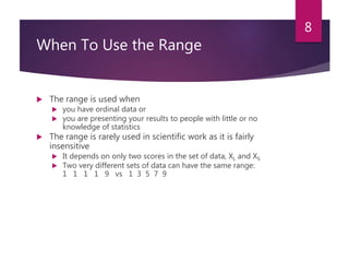
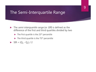
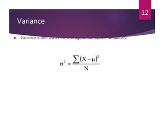
This document defines and explains various measures of dispersion used in statistics, including range, semi-interquartile range (SIR), variance, standard deviation, skew, and kurtosis. It provides formulas for calculating each measure and discusses how to interpret the results, such as how skew values indicate the direction and degree of asymmetry and how kurtosis compares the spread of a distribution to a normal distribution. The purpose of measuring dispersion is to understand the variability and shape of distributions for purposes like determining reliability and facilitating other statistical analyses.

1. Measures of
Dispersion
DR. JULEE
1

2. Definition
 Measures of dispersion are descriptive statistics that
describe how similar a set of scores are to each other
 The more similar the scores are to each other, the lower the
measure of dispersion will be
 The less similar the scores are to each other, the higher the
measure of dispersion will be
 In general, the more spread out a distribution is, the larger
the measure of dispersion will be
2

3. Measures of Dispersion
 Which of the
distributions of scores
has the larger
dispersion?
0
25
50
75
100
125
1 2 3 4 5 6 7 8 9 10
0
25
50
75
100
125
1 2 3 4 5 6 7 8 9 10
3
The upper distribution
has more dispersion
because the scores are
more spread out
That is, they are less
similar to each other

4. Measures of Dispersion
 There are three main measures of dispersion:
 The range
 The semi-interquartile range (SIR)
 Variance / standard deviation
 Mean Deviation and average deviation
 The Lorenz curve
4

5. Properties of Good measure of
Variation
 It should be simple to understand
 It should be easy to compute
 It should be based on each and every item of the
distribution
 It should not be unduly affected by the extreme items
 It should be rigidly defined.
5

6. Significance of Measuring
Variation
 There are four basic purpose
 To determine the reliability of an average
 To serve as the basis for the control of the variability
 To compare two or more series with regard to their
variability
 To facilitate the use of other statistical measures.
6

7. The Range
 The range is defined as the difference between the
largest score in the set of data and the smallest score in
the set of data, XL - XS
 What is the range of the following data:
4 8 1 6 6 2 9 3 6 9
 The largest score (XL) is 9; the smallest score (XS) is 1; the
range is XL - XS = 9 - 1 = 8
7

8. When To Use the Range
 The range is used when
 you have ordinal data or
 you are presenting your results to people with little or no
knowledge of statistics
 The range is rarely used in scientific work as it is fairly
insensitive
 It depends on only two scores in the set of data, XL and XS
 Two very different sets of data can have the same range:
1 1 1 1 9 vs 1 3 5 7 9
8

9. The Semi-Interquartile Range
 The semi-interquartile range (or SIR) is defined as the
difference of the first and third quartiles divided by two
 The first quartile is the 25th percentile
 The third quartile is the 75th percentile
 SIR = (Q3 - Q1) / 2
9

10. SIR Example
 What is the SIR for the
data to the right?
 25 % of the scores are
below 5
 5 is the first quartile
 25 % of the scores are
above 25
 25 is the third quartile
 SIR = (Q3 - Q1) / 2 = (25
- 5) / 2 = 10
2
4
6
 5 = 25th
%tile
8
10
12
14
20
30
 25 = 75th
%tile
60
10

11. When To Use the SIR
 The SIR is often used with skewed data as it is insensitive
to the extreme scores
11

12. Variance
 Variance is defined as the average of the square deviations:
12
 
N
X
2
2  




13. What Does the Variance Formula
Mean?
 First, it says to subtract the mean from each of the scores
 This difference is called a deviate or a deviation score
 The deviate tells us how far a given score is from the typical,
or average, score
 Thus, the deviate is a measure of dispersion for a given score
13

14. What Does the Variance Formula
Mean?
 Why can’t we simply take the average of the deviates? That is, why isn’t
variance defined as:
14
 
N
X
2  



This is not the formula
for variance!

15. What Does the Variance Formula
Mean?
 One of the definitions of the mean was that it always
made the sum of the scores minus the mean equal to 0
 Thus, the average of the deviates must be 0 since the sum
of the deviates must equal 0
 To avoid this problem, statisticians square the deviate
score prior to averaging them
 Squaring the deviate score makes all the squared scores
positive
15

16. What Does the Variance Formula
Mean?
 Variance is the mean of the squared deviation scores
 The larger the variance is, the more the scores deviate, on
average, away from the mean
 The smaller the variance is, the less the scores deviate, on
average, from the mean
16

17. Standard Deviation
 When the deviate scores are squared in variance, their unit of measure is
squared as well
 E.g. If people’s weights are measured in pounds, then the variance of the weights
would be expressed in pounds2 (or squared pounds)
 Since squared units of measure are often awkward to deal with, the square root
of variance is often used instead
 The standard deviation is the square root of variance
17

18. Standard Deviation
 Standard deviation = variance
 Variance = standard deviation2
18

19. Computational Formula
 When calculating variance, it is often easier to
use a computational formula which is
algebraically equivalent to the definitional
formula:
 
 
N
N
N X
X
X
2
2
2
2  


 



19
2 is the population variance, X is a score,  is the
population mean, and N is the number of scores

20. Computational Formula Example
X X2
X- (X-)2
9 81 2 4
8 64 1 1
6 36 -1 1
5 25 -2 4
8 64 1 1
6 36 -1 1
 = 42  = 306  = 0  = 12
20

21. Computational Formula Example
 
2
6
12
6
294
306
6
6
306
N
N
42
X
X
2
2
2
2











 
2
6
12
N
X
2
2



 


21

22. Variance of a Sample
 Because the sample mean is not a perfect
estimate of the population mean, the formula for
the variance of a sample is slightly different from
the formula for the variance of a population:
 
1
N
X
X
s
2
2


 
22
s2 is the sample variance, X is a score, X is the
sample mean, and N is the number of scores

23. Measure of Skew
 Skew is a measure of symmetry in the distribution of scores
23
Positive Skew Negative Skew
Normal (skew =
0)

24. Measure of Skew
 The following formula can be used to determine skew:
24
 
 
N
N
X
X
X
X
s 2
3
3
 
 


25. Measure of Skew
 If s3 < 0, then the distribution has a negative skew
 If s3 > 0 then the distribution has a positive skew
 If s3 = 0 then the distribution is symmetrical
 The more different s3 is from 0, the greater the skew in
the distribution
25

26. Kurtosis
(Not Related to Halitosis)
 Kurtosis measures whether the scores are spread out more or less than
they would be in a normal (Gaussian) distribution
26
Mesokurtic
(s4 = 3)
Leptokurtic (s4 > 3) Platykurtic (s4 < 3)

27. Kurtosis
 When the distribution is normally distributed, its kurtosis
equals 3 and it is said to be mesokurtic
 When the distribution is less spread out than normal, its
kurtosis is greater than 3 and it is said to be leptokurtic
 When the distribution is more spread out than normal, its
kurtosis is less than 3 and it is said to be platykurtic
27

28. Measure of Kurtosis
 The measure of kurtosis is given by:
28
 
N
N
X
X
X
X
s
4
2
4

 

















29. s2, s3, & s4
 Collectively, the variance (s2), skew (s3), and kurtosis (s4)
describe the shape of the distribution
29