This document presents an adaptive Kalman filter for estimating human body orientation using micro-sensors. The filter uses quaternions to represent orientation to avoid singularities. It includes motion acceleration in the state vector to compensate for interference of body motion on gravity measurements. Additionally, it adapts the process noise covariance based on sensor signal variations to optimize performance under human motion. Experiments showed this algorithm had less error than existing methods and that including motion compensation and adaptive mechanisms improved accuracy of human motion capture.

1. Adaptive Kalman Filter for Orientation Estimation
in Micro-sensor Motion Capture
Shuyan Sun1,2, Xiaoli Meng1,2, Lianying Ji1,2, Zhipei Huang1 and Jiankang Wu1,2
1.Graduate University of Chinese Academy of Sciences, Beijing, China
2.China-Singapore Institute of Digital Media, Singapore
{sunshuy09b, mengxiaoli07}@mails.gucas.ac.cn, {jilianying, zhphuang, jkwu}@gucas.ac.cn
Abstract—One of the biggest challenges in micro-sensor motion
capture is the drift problem caused by integration of angular
rates to obtain orientation estimation. To reduce the drift,
existing algorithms make use of gravity and earth magnetic field
measured by accelerometers and magnetometers. Unfortunately,
the gravity measurement can be strongly interfered by human
motion acceleration. This paper presents a quaternion-based
adaptive Kalman filter for drift-free orientation estimation. In
this filter, the motion acceleration associated with the quaternion
is included in the state vector, to compensate the effects which
human body motion may have on the reliability of gravity
measurement. Moreover, the process noise covariance is adapted
based on the variation of sensor signals, to optimize the perfor-
mance under human motion existence. The final experiments
show that the proposed algorithm has least error compared
with the existing methods, and the use of motion acceleration
compensation together with the adaptive mechanism can improve
the accuracy of human motion capture.
Keywords: Sensor fusion, Kalman filter, adaptive mecha-
nism, human motion capture, drift.
I. INTRODUCTION
Human motion capture (Mocap) has wide applications in
many areas, such as virtual reality, interactive game and
learning, animation and film special effects, etc. Among all
the motion capture techniques, optical motion capture is one
of the most mature techniques. However, an optical human
motion capture system usually has certain limitations: it needs
multiple high speed and high resolution cameras structured and
calibrated in a dedicated studio, which restricts applications
into a studio-like environment; the system is quite complex
and there is a huge amount of data to be processed; moreover,
an optical motion capture system is usually very expensive
and inconvenient to most applications.
With the rapid advances of micro-electro-mechanical sys-
tems (MEMS) sensors, the research on human motion cap-
ture using micro-inertial sensors becomes more attractive. In
Micro-sensor Motion capture (MMocap), miniature sensors
are attached to body segments. Segment orientation can be
estimated from the fusion of sensory data. Based on the
estimated orientation, together with the length of each segment
and the arranging relationship between segments, the motion
of the whole body can be obtained. MMocap has no line-
of-sight requirements, and no emitters to install [1]. Thus,
MMocap systems can be applied in a variety of applications
where a studio-like environment is not necessary. The motion
measurements in MMocap are relatively direct, and the system
is relatively simple, at least not as complicated as optical
Mocap systems. Moreover, a MMocap system costs much
lower than that based on the optical Mocap.
However, there are technical challenges due to its inherit
characteristics in MMocap. One of the biggest challenges is
the data fusion of three types of miniature sensors contained
in a micro Sensor Measurement Unit (SMU), namely, 3D
micro-gyroscope, 3D accelerometer and 3D magnetometer. In
MMocap there is a SMU node attached to each body segment
to be captured. The gyroscope measures angular rates, by
the integration of which orientation of that body segment
can be obtained. As the result of integration, the errors also
accumulate. This results in a drift over a period of time.
Because the drift of each body segment is most likely toward
a different direction, leading to inconsistency issues when
forming the whole body motion. In order to reduce the drift
in the data fusion algorithms, the magnetometer, based on the
principle of a compass to measure the earth magnetic field,
is employed to measure azimuth angle or rotations about the
vertical axis. The accelerometer measures the gravity vector
relative to the sensor coordinate system, and allows accurate
determination of pitch and roll angle. However, there will also
be problems if the body acceleration cannot be neglected with
comparison to gravity. The data from these three kinds of
sensors are usually fused in an algorithm to “eliminate” the
drift and to derive the orientation estimation.
There are many fusion algorithms to obtain orientation from
gyroscope, accelerometer and magnetometer signals. Foxlin et
al. [2] proposed a complementary separate-bias Kalman filter,
which was designed for head tracking applications. Yun et al.
presented a factored quaternion algorithm (FQA) [3], which
restricts the use of magnetic data to the determination of the
azimuth angle. They illustrated that FQA was computationally
more efficient and the magnetic variations caused only azimuth
errors in attitude estimation. Roetenberg et al. [4] described
a complementary Kalman filter design, which compensated
the magnetic disturbance by estimating the disturbance error
and adaptively changing the measurement covariance based on
the disturbance estimation. Kraft [5] described an unscented
quaternion-based Kalman filter for real-time estimation of a
rigid body orientation. Sabatini [6] developed a quaternion
based extended Kalman filter (EKF), where the measurement
noise covariance matrix was adapted, to guard against the
interference from body motion acceleration and temporary
14th International Conference on Information Fusion
Chicago, Illinois, USA, July 5-8, 2011
978-0-9824438-3-5 ©2011 ISIF 1693

2. magnetic disturbance. Young [7] presented simulations of
an algorithm for estimating linear acceleration of wireless
inertial measurement units based on body model constraints,
to improve the accuracy of inertial motion capture. Among
all the studies mentioned above, Roetenberg [4] compen-
sated magnetic disturbance, but rotation matrix of orientation
representation suffers from the singularity problem; Sabatini
[6] adapted the measurement noise covariance matrix, to
guard against the interference from body motion acceleration
and temporary magnetic disturbance, but the long-time and
continuous interference cannot be easily guarded; the FQA
[3] restricted the use of the magnetometer, and the inference
from magnetic disturbance to roll and pitch was removed, but
the motion acceleration cannot be removed.
Considering the state-of-the-art of MMcap, we propose a
quaternion-based Adaptive Kalman filter (AKF) for motion es-
timation using miniature SMU’s. The novelty of the AKF is the
quaternion-based filter structure and the adaptive mechanism,
which can compensate interference from human acceleration
adaptively and can estimate orientation without either the drift
or the singularity problem. One of the contributions of this
paper is: in the designed AKF, quaternions are selected to
represent the rotation and orientation of each body segment,
for they do not suffer from the singularity problem; the motion
acceleration is also included in the state vector, to compensate
the effects which human body motion may have on the
reliability of gravity measurement. Another contribution of this
paper is the adaptive mechanism. To optimize the performance
under human motion existence, this filter fuses sensory data
adaptively by adapting the process noise covariance based on
the variation of sensor signals. The good performance of the
experimental results has shown the feasibility and effectiveness
of the proposed algorithm.
The rest of the paper is organized as follows. Section II
describes the quaternion-based AKF for sensor fusion. Section
III presents the experimental results. Finally, conclusions and
future work are given in Section IV.
II. PROPOSED ADAPTIVE KALMAN FILTER
The proposed AKF takes a quaternion to represent the
orientation of each body segment. Under the filtering frame-
work, the integrated quaternion from gyroscope signals is
corrected by the gravity and earth magnetic direction for
drift-free orientation, and the motion acceleration is compen-
sated adaptively to guard against the interference from body
motion to gravity measurement. This section first describes
the quaternion representation, which is followed by the filter
process model and the measurement model employed by the
AKF. Then the adaptive mechanism and the filter design are
explained.
A. Quaternion representation
In MMocap, a SMU is fixed on a body segment. Before the
analysis it is necessary to define the coordinate systems. First,
there exists a Global Coordinate System (GCS) which is earth
related and time invariant. GCS is taken as the reference frame.
Second, a Body Coordinate System (BCS) is attached to the
body segment which is time variant coinciding with segment
motion. The orientations between GCS and BCS are what to be
determined. The Sensor Coordinate System (SCS) is defined
by the SMU itself and also coincides with segment motion.
Since the SMU is rigidly attached to the body segment, the
orientation between BCS and SCS is a constant offset. For
the convenience of analysis, it is assumed that SCS coincides
with BCS all the time, and GCS, BCS, and SCS are denoted
as the reference frame, the body frame and the sensor frame,
respectively.
Quaternions are selected to represent the rotation and orien-
tation of the body segment. A quaternion consists of a vector
part e=(q1,q2,q3)T
∈R3
and a scalar part q4∈R [8], where the
superscript T denotes the transpose of a vector:
q = (eT
, q4)T
=
⎛
⎜
⎜
⎝
q1
q2
q3
q4
⎞
⎟
⎟
⎠ (1)
The quaternion can be used for the representation of the
transformation relationship between the reference frame and
the body frame, e.g., any given vector r∈R3
in the reference
frame can be rotated into the body frame by a unit quaternion
q:
b = C(q)r (2)
where the vector b∈R3
is the representation in the body
frame of vector r, and C(q) is the orientation matrix of the
transformation from the reference frame to the body frame [8]:
C(q) = (q2
4 − eT
e)I3 + 2eeT
− 2q4[e×] (3)
where I3 denotes 3×3 identity matrix, and the operator [e×]
represents the standard vector cross-product:
[e×] =
⎛
⎝
0 −q3 q2
q3 0 −q1
−q2 q1 0
⎞
⎠ (4)
It is well-known that quaternions satisfy the following
vector differential equation [8]:
d
dt
q =
1
2
Ω[ω]q (5)
where Ω[ω] is a 4x4 skew symmetric matrix:
Ω[ω] =
−[ω×] ω
−ωT
0
(6)
And ω is the angular velocity of the body frame relative to
the reference frame, resolved in the body frame:
ω =
⎛
⎝
ωx
ωy
ωz
⎞
⎠ (7)
with [ω×] representing cross product operator as in (4).
1694

3. Given the sampling interval Δ, if the angular velocity ωt
measured at time instants tΔ is constant in the interval [(t-
1)Δ,tΔ], then equation (5) can be extended into the discrete-
time model:
qt = exp
1
2
Ω[ωt]Δ qt−1 (8)
However, the validity of (8) is subject to the assumption that
the angular velocity ωt is constant in the interval [(t-1)Δ,tΔ].
B. Process model
The process model employed by the filter governs the
dynamic relationship between states of two successive time
steps. In what follows, the process dynamic transition function
and the noise model will be derived.
As mentioned above, the gyroscope measures the angular
velocity with bias and noise,
yG,t = ωt + hG,t + vG,t (9)
where vG,t is the gyroscope noise modelled as a Gaussian
noise, N(0,ΣG), and hG,t is the bias vector (assumed to
be null). Here the subscript ‘G’ means gyroscope, and the
subscript t denotes time. Substituting (9) into (8) and taking
the angular velocity error into account, we have:
qt = exp
1
2
Ω[yG,t − hG,t − vG,t]Δ qt−1
≈ exp
1
2
Ω[yG,t]Δ qt−1 −
1
2
Ξt−1vG,t
= Atqt−1 + wq,t
(10)
where At is the dynamic transition matrix:
At = exp
1
2
Ω[yG,t]Δ (11)
and wq,t is a random noise:
wq,t = −
1
2
Ξt−1vG,t (12)
Here wq,t is modelled as a zero mean Gauss distribution, with
covariance matrix:
Qq,t =
Δ
2
2
Ξt−1ΣGΞT
t−1 (13)
where
Ξt =
[et×] + qt,4I3
−eT
t
(14)
The equation (10) describes the quaternion dynamic tran-
sition against time. It is a first-order approximation in vG,t
and Δ of the true process (8) [8], when the true angular
velocity to be used in (8) cannot be obtained in practice, but it
is rather measured. The approximation is achieved under the
assumption that the gyroscope measurement noise vG,t and
the sampling interval Δ are small enough that a first order
approximation of the transition matrix is possible.
The accelerometer measures accelerations. When human
motion occurs, there will be signals of human motion accel-
eration contained in accelerometer measurements. The motion
acceleration is modelled as a first-order low-pass filtered white
noise process according to:
at = cat−1 + wa,t (15)
where at is the motion acceleration, c is a constant, and wa,t
is a random noise and is modelled as a zero mean Gauss
distribution, whose covariance matrix is Q=σ2
a,tI3.
After the derivation of dynamic relationship of quaternion
and acceleration vectors between two successive time steps,
the final process model is obtained. The state vector xt of the
filter is composed of the rotation quaternion and the motion
acceleration, which is given by:
xt =
qt
at
(16)
And the state transition equation is:
xt = F xt−1 + wt
=
At O4×3
O3×4 cI3
xt−1 +
wq,t
wa,t
(17)
where At and wq,t are given by (11) and (12) respectively,
while O stands for zero matrix, and other parameters are the
same as above. In this work, it is assumed that wq,t and
wa,t are not correlated with each other, thus the process noise
covariance matrix Qt will have the following expression:
Qt =
Δ
2
2
Ξt−1ΣGΞT
t−1 O4×3
O3×4 Qa,t
(18)
where Qa,t=σ2
a,tI is adapted as shown in below.
In this process model, the gyroscope signal is used as the
input in the system model, thus the orientation quaternion of
each time step can be updated with the newest angular signals
without the delay of one time step. And the uncertainties of
the angular rates are considered in the system equation by the
process noise as shown in (10).
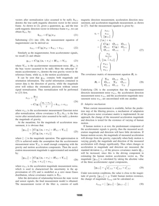
C. Measurement model
The measurement model employed by the filter governs the
relationship between the state vector and sensor signals. From
magnetometer signals, we obtain
yM,t = BM,t + HM,t + VM,t (19)
where VM,t is the magnetometer measurement noise. HM,t is
the bias vector (assumed to be null). Here the subscript ‘M’
means magnetometer. BM,t denotes the earth magnetic field
plus disturbance, which is sampled in the sensor frame. In this
work, the interference from magnetic disturbance is ignored. It
can be seen that yM,t contains both magnitude and orientation
information. The useful information contained in sensor data is
the direction of earth magnetic field, while the magnitude error
will reduce the orientation precision without sensor signal
normalization. Thus normalization will be performed to (19)
first,
zM,t = bM,t + hM,t + vM,t (20)
where vM,t is the magnetometer measurement Gaussian noise
after normalization, whose covariance is ΣM ; hM,t is the bias
1695

4. vectors after normalization (also assumed to be null); bM,t
denotes the true earth magnetic direction vector in the sensor
frame. As shown in (2), given a quaternion, qt, and the true
earth magnetic direction vector in reference frame rM , we can
obtain bM,t by:
bM,t = C(qt)rM (21)
Substituting (21) into (20), the measurement equation of
magnetometer can be derived as:
zM,t = C(qt)rM + hM,t + vM,t (22)
Similarly as the magnetometer, from accelerometer signals,
we recall (2) and obtain:
yA,t = C(qt)(at + rA) + HA,t + VA,t (23)
where VA,t is the accelerometer measurement noise. HA,t is
the bias vector (assumed to be null). Here the subscript ‘A’
means accelerometer. rA denotes the true gravity vector in the
reference frame, while at is the motion acceleration.
It can be seen that yA,t contains both magnitude and
orientation information. The useful information contained in
sensor data is the direction of gravity, while the magnitude
error will reduce the orientation precision without sensor
signal normalization. Thus normalization will be performed
to (23) first,
zA,t =
yA,t
g
= C(qt)
at + rA
g
+ hA,t + vA,t
(24)
where vA,t is the accelerometer measurement Gaussian noise
after normalization, whose covariance is ΣA; hA,t is the bias
vector after normalization (also assumed to be null); g denotes
the magnitude of gravity.
At the meantime, for the magnitude of acceleration mea-
surement, it is obvious that:
yA,t = C(qt)(at + rA) + HA,t + VA,t
≈ C(qt)(at + rA)
(25)
where · is the magnitude operation. The approximation in
(25) is achieved under the assumption that the accelerometer
measurement noise VA,t is small enough comparing with the
gravity and motion acceleration components. Then the accel-
eration measurement magnitude is approximated and modelled
by:
yA,t = C(qt)(at + rA) + HA,t + VA,t
= (at + rA) + vN,t
(26)
where vN,t is the acceleration magnitude measurement noise,
which is used to characterized the uncertainty in the ap-
proximation of (25) and is modelled as a zero mean Gauss
distribution, whose covariance matrix is ΣN .
After the derivation of relationship between the state vector
and sensor signals, the final measurement model is obtained.
The measurement vector of the filter zt consists of earth
magnetic direction measurement, acceleration direction mea-
surement, and acceleration magnitude measurement, as shown
in (27). And the measurement equation is given by:
zt =
⎛
⎝
zM,t
zA,t
yA,t
⎞
⎠
= f(xt) + vt
=
⎛
⎝
C(qt) O3×3 O3×1
O3×3 C(qt) O3×1
O1×3 O1×3 1
⎞
⎠
·
⎛
⎝
rM
at+rA
g
(at + rA)
⎞
⎠
+
⎛
⎝
vM,t
vA,t
vN,t
⎞
⎠
(27)
The covariance matrix of measurement equation Rt is:
Rt =
⎛
⎝
ΣM O3×3 O3×1
O3×3 ΣA O3×1
O1×3 O1×3 ΣN
⎞
⎠ (28)
Underlying (28) is the assumption that the magnetometer
direction measurement noise vM,t, the acceleration direction
measurement noise vA,t, and the acceleration magnitude mea-
surement noise vN,t are uncorrelated with one another.
D. Adaptive mechanism
When current measurement is available, before the predic-
tion step of the filtering process, a mechanism of adaptation
of the process noise covariance matrix is implemented. In our
approach, the change of the measured acceleration magnitude
and direction is tested for the existence of varying of human
motion.
If human motion is at rest, the predominant component of
the accelerometer signals is gravity, thus the measured accel-
eration magnitude and direction will have little deviations. If
human motion occurs, the magnitude of measured acceleration
will diverge from the gravity; especially when body motion is
varying greatly, the magnitude and direction of the measured
acceleration will change significantly. Thus when changes in
acceleration in magnitude and direction are measured, the
standard deviation σa,t of the process covariance matrix Qa,t
will be increased, since this is the driving component in
estimating the human motion acceleration vector at. The
magnitude yA,t is calculated by taking the absolute value
of the three accelerometer signal components,
yA,t = y2
x,A,t + y2
y,A,t + y2
z,A,t (29)
Under non-motion conditions, the value is close to the magni-
tude of gravity yA,t = g. Under human motion existence,
the change of magnitude δmag can be calculated as:
δmag = yA,t − yA,t−1 (30)
1696

5. In order to calculate the change of direction δdir, the measured
accelerometer signals should be expressed in the reference
frame firstly, then the arc cosine functions between two
successive sampling accelerometer signals will be taken:
δdir = arccos
C−1
(q−
t )yA,t · (q+
t−1)yA,t−1
yA,t · yA,t−1
(31)
The term C−1
(q−
t )yA,t is the predicted acceleration in the
reference frame, where the superscript – and + stand for “a
priori estimate” and “a posteriori estimate” respectively, and
C−1
(q) is the orientation matrix representing the transforma-
tion from the sensor frame to the reference frame.
If δmag and δdir are close to zeros, human motion acceler-
ation is absent or the change of acceleration is not significant;
when their values are away from zeros, the change of human
motion acceleration takes place, thus at should change by
updating σa,t:
σa,t =
σa,0, δdir < εdir δmag < εmag
σa,mag · δmag + σa,dir · δdir, otherwise
(32)
where σa,0, σa,mag, and σa,dir are predefined parameters,
while the latter two determine the contributions of the change
in magnitude and direction. Then the process noise covariance
matrix Qa,t=σ2
a,tI3 is adapted.
The proposed adaptive mechanism aims at precluding the
human motion acceleration from influencing the filter be-
havior, when detected changes of motion acceleration are
characterized by variation of measured acceleration magnitude
or direction. In this regard, the influence from the bias vectors
hA,t and hM,t is ignored, which can be found in literatures
[4] [6].
Given the process model through (16-18), the measurement
model (27-28) and the adaptive mechanism (29-32), the ori-
entation of each body segment can be estimated without drift.
Under the filtering framework, the integrated quaternion from
gyroscope signals is corrected by the gravity and earth mag-
netic direction, and the motion acceleration is compensated
adaptively to guard against the interference from body motion
to gravity measurement.
Because of the nonlinear nature about the state vector of
(27), the standard Kalman filter cannot be used here directly,
since the standard Kalman filter can only deal with linear
models with Gaussian noise distribution. In this work, the
Unscented Kalman Filter (UKF) is selected to deal with the
nonlinearity of (27). The detailed UKF equations can be found
in [9].
III. EXPERIMENTAL RESULTS
For the evaluation of the proposed algorithm, two rep-
resentative experiments were carried out. In the first one,
simulation tests were performed during which inertial sensor
data were generated from existing motion capture data. Use
of simulated data allows a wide variety of motions to be
tested. In the second one, a miniature sensor was translated
and rotated under motion acceleration to test the performance
of the algorithm quantitatively.
Figure 1. The relationship between pelvis, femur, tibia and foot segments
A. Computer simulations
In the first experiment, simulation tests were performed
during which inertial sensor data were generated from existing
motion capture data, while the data source for evaluation were
taken from the Carnegie Mellon University motion capture
data base [10]. The data in the CMU database were captured
by an optical tracking system (Vicon Oxford Metrics, Oxford,
U.K.), containing the root position and relative orientation data
of each body segment saved in the ASF/AMC format files.
In order to reduce processing times, and to simplify result
presentation at the same time, the motion data in ASF/AMC
format were pre-processed to remove the upper body, leaving
the pelvis, and the left and right femur, tibia and foot. The
relationship between there segments are shown in Figure 1.
From the root position and relative orientation data, the
position, velocity, acceleration, orientation, and angular veloc-
ity data of each joint can be calculated. Motion accelerations
and angular velocities were calculated by applying the central
difference technique to the position and rotation data. The
simulated earth magnetic field vector was generated by rotating
a reference magnetic vector from the reference frame into the
sensor frame by the true orientation data.
Before the simulated sensor data and motion data can be
used, a low-pass Butterworth filter with a cutoff at 20Hz was
used on the motion capture data to remove high frequency
noise from the optical data which would otherwise dominate
numerical estimates of derivative functions. In this simulation,
virtual sensors were assumed to be attached to on human body
segments. The sensor of the pelvis was collocated with the
joint, while other virtual sensors were mapped onto the bone
halfway between the proximal and distal joints, e.g. the left
tibia sensor was located halfway between the knee and ankle
joints [7].
Two motion capture data were selected for evaluation during
simulation. These were: 16 15, 470 frames, contain three
walking gait cycles; 49 02, 2085 frames, contain motion of
jumping up and down, hopping on one foot.
All data were sampled at 120Hz. The simulated sensor
data were corrupted by Gaussian colored noise, while the
noise was processed by a low-pass Butterworth filter with a
cutoff at 60Hz, and the standard deviations of the sensor noise
sources of accelerometers, magnetometers and gyroscopes
were given as 0.3m/s2
, 0.0003full scale and 0.03125rad/s,
respectively [7]. In addition to sensor noise, the effects of rate
1697

6. gyroscope bias were modeled. Gyroscope bias was modeled as
a constant offset normally distributed in each gyroscope axis
with standard deviation of 0.03125 rad/s. In the simulation the
initial orientations of the virtual sensors were set to the true
orientation of the joint [7].
For the convenience of discussion, in what following, our
algorithm was named as ‘A’, for the meaning of ‘Adaptive’.
Also, three other methods were implemented, which were
named as ‘B’, ‘C’ and ‘D’. Method B is a quaternion-based
UKF filtering method without the consideration of compen-
sation of human motion acceleration. Method C is the FQA
algorithm [3]. And method D integrates angular rates to obtain
orientation directly. Also, for the convenience of evaluation,
quaternions from fusion methods were transformed into Euler
angles, i.e., roll, pitch and yaw angle.
The evaluation performance metrics were based on comput-
ing the error angle θ between the true orientation and estimated
orientation:
θ = 2arccos q−1
true⊗q+
(33)
where qtrue and q+
are the true and estimated quaternions,
respectively. The evaluation metrics were given by the root-
mean-square error RMSEθ. Besides, the true quaternions and
estimated quaternions from these four methods were operated
on the unit vectors ru of the reference frame using (2)
separately:
btrue = C (qtrue) ru
b+
= C q+
ru
ru =
⎧
⎪⎨
⎪⎩
(0 0 1)T
(0 1 0)T
(1 0 0)T
(34)
where ru represents the unit vectors of the reference frame;
btrue represents the true unit vectors, i.e., the result unit
vectors from the operation by the true quaternions; b+
rep-
resents the estimated vectors, i.e., the result vectors from
the operation by the estimated quaternions. The RMS error
between the true vectors btrue and the estimated vectors b+
,
i.e, RMSE(btrue − b+
), were also calculated and provided.
The accuracy comparison results of the four different orien-
tation filter implementations are summarized in Table I-IV, for
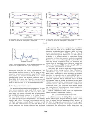
the walking and jumping trials respectively. The tables show
the mean RMSEs of angles, together with the RMSE of unit
vectors. The angles of roll, pitch, and yaw against time of the
rfoot segment are shown in Figure 2. Also the corresponding
human motion acceleration is shown in Figure 3.
From Figure 2-3, it can be seen that without correction
from fusion of other sensing, Euler angles integrated directly
from gyroscope signals of method D become more and more
inaccurate with the accumulation of time. This is the drift
problem. FQA results of method C fluctuate greatly and have
peaks under motion acceleration; UKF results of method B do
not fluctuate as much as method C under motion acceleration.
Also, the results from Table I-II for the walking trial show
that method A has the smallest RMSE, and achieved the best
Table I
RMSES (DEGREES) OF ANGLES BETWEEN THE TRUE AND ESTIMATED
QUATERNIONS, PROVIDED BY THE FOUR FILTERING METHOD
RESPECTIVELY, FOR THE WALKING TRIAL
RMSE angle(deg) A B C D
pelvis 1.1551 3.6880 6.6846 6.6054
lfemur 1.2346 3.7777 6.7287 10.6357
ltibia 1.1383 3.6240 6.8067 12.6702
lfoot 1.8684 3.5994 6.7267 29.1181
rfemur 1.5331 3.8053 6.7538 15.6112
rtibia 1.2514 3.6951 6.7096 20.6552
rfoot 1.9833 3.5498 6.5779 39.8305
Table II
RMSE OF UNIT VECTORS BETWEEN THE ONES OPERATED BY THE TRUE
QUATERNIONS AND THE ONES BY THE ESTIMATED QUATERNIONS, FOR
THE WALKING TRIAL
RMSE vectors A B C D
pelvis 0.0167 0.0528 0.0941 0.0931
lfemur 0.0181 0.0545 0.0946 0.1481
ltibia 0.0164 0.0522 0.0954 0.1783
lfoot 0.0264 0.0522 0.0941 0.3689
rfemur 0.0215 0.0537 0.0951 0.2199
rtibia 0.0178 0.0522 0.0944 0.2856
rfoot 0.0293 0.0505 0.0927 0.4962
Table III
RMSES (DEGREES) OF ANGLES BETWEEN THE TRUE AND ESTIMATED
QUATERNIONS, PROVIDED BY THE FOUR FILTERING METHOD
RESPECTIVELY, FOR THE JUMPING TRIAL
RMSE angle(deg) A B C D
pelvis 2.3606 29.6633 43.2127 23.2081
lfemur 3.7389 30.3777 46.0423 62.3486
ltibia 3.6079 30.6670 47.6567 22.0324
lfoot 3.6771 32.1724 46.0113 28.0149
rfemur 3.2752 31.4083 45.5018 17.7316
rtibia 2.5261 30.8450 47.6191 32.1052
rfoot 2.3694 30.5894 45.8387 34.4556
Table IV
RMSE OF UNIT VECTORS BETWEEN THE ONES OPERATED BY THE TRUE
QUATERNIONS AND THE ONES BY THE ESTIMATED QUATERNIONS, FOR
THE JUMPING TRIAL
RMSE vectors A B C D
pelvis 0.0349 0.3672 0.4473 0.3132
lfemur 0.0482 0.3695 0.4475 0.5251
ltibia 0.0484 0.3708 0.4479 0.2932
lfoot 0.0464 0.3761 0.4467 0.3733
rfemur 0.0466 0.3638 0.4473 0.2454
rtibia 0.0363 0.3666 0.4468 0.3973
rfoot 0.0345 0.3617 0.4470 0.4312
1698

7. 750 800 850 900
−100
0
100
200
Roll(deg)
True
D
A
750 800 850 900
−60
−40
−20
0
20
Pitch(deg)
750 800 850 900
−20
0
20
40
Yaw(deg)
time (0.0083s)
(a) Euler angles of the true value, method A and D estimates from time step
701 to time step 900, for the rfoot segment of jumping trial
750 800 850 900
−100
0
100
200
Roll(deg)
True
B
C
750 800 850 900
−60
−40
−20
0
20
Pitch(deg)
750 800 850 900
−20
0
20
40
Yaw(deg)
time (0.0083s)
(b) Euler angles of the true value, method B and C estimates from time step
701 to time step 900, for the rfoot segment of jumping trial
Figure 2.
750 800 850 900
0
20
40
60
Accmagnitude(m/s2
)
time step (0.0083s)
Figure 3. Acceleration magnitude of the true motion acceleration from time
step 701 to time step 900, for the rfoot segment of jumping trial
performance among the four filtering implementations. The
reason for the improved accuracy of A is its ability to com-
pensate the human motion acceleration adaptively. The results
of the jumping trial, presented in Table III-IV, show a similar
tendency to the walking trial. However, comparing Table I-
II and Table III-IV, along with Figure 2-3, we can see that
the greater human motion acceleration during motion capture
results in increased error for all the filter implementations.
B. Data fusion with miniature sensors
The second experiment investigates the stability of the filter
under motion acceleration using single SMU sensor, when
the sensor was rotated for –90◦
and +90◦
along Z axis. The
sensor SMU used for this experiment was the micro-sensor
chip ADIS16405 which is produced by the Analog Devices.
The sensor SMU consists of a tri-axis accelerometer, a tri-
axis gyroscope and a tri-axis magnetometer. The sampling
frequency was 100Hz. The sensor was first placed statically
with Z-axis pointing up vertically. Then it was rotated around
Z axis for –90◦
and then rotated back for +90◦
. During the
rotation, translation with motion acceleration was performed
at the same time. This process was repeated for several times
with a total time length of 40s. The Euler angles from these
estimation methods are shown in Figure 4, while local zoom
results from time step 451 to 1080 are shown in Figure 5.
The acceleration magnitude of time slices 451-1080 is present
in Figure 6. As shown in Figure 6, when human motion
acceleration is absent, the measured acceleration magnitude
from the sensor is close to the magnitude of gravity; however
when the motion acceleration occurs, the magnitude will
diverge from the magnitude gravity. Given the ground truth
of zeros, the estimation RMSE of angles along X and Y axes
are calculated and summarized in Table V.
From Figure 4-6, it can be seen that without correction
from fusion of other sensing, results of B and C fluctuate for
all of the three angles under motion acceleration introduced.
From Table V and Figure 4-6, it can be seen that the proposed
algorithm, i.e., method A, has the smallest RMSE, and does
not fluctuate much under motion acceleration. Also it can be
seen from Figure 4-6 that the orientation error of B and C
will increase when the motion acceleration became larger,
which is consistent with the simulation experiment. But the
orientation error of A does not increase much when the motion
acceleration grows. This is because during human motion,
the compensation of the accelerometer signals in method A
improves the accuracy of the filter.
From the comparison of these results, our algorithm has
shown its accuracy, stability and efficiency.
IV. CONCLUSIONS AND FUTURE WORK
In order to overcome the drift problem in micro-sensor
human motion capture, this paper presents an adaptive Kalman
filter, to estimate drift-free orientation of body segments. In
this filter, the integrated quaternion from gyroscope signals
is corrected by the gravity and magnetic direction from
accelerometer and magnetometer signals, respectively. The
1699

8. Table V
RMSE ANGLES OF EACH METHOD
Approach Roll (deg) Pitch (deg)
A 0.6506 0.7537
B 7.1081 9.2586
C 19.0836 24.4278
D 20.4569 16.0910
1000 2000 3000 4000
0
20
40
60
Roll(deg)
A
B
C
1000 2000 3000 4000
−50
0
50
Pitch(deg)
1000 2000 3000 4000
−100
−50
0
50
Yaw(deg)
time (0.01s)
Figure 4. Euler angles (true value of X and Y angles are zeros), where the
sensor was rotated about Z axis with translation acceleration. Provided by the
filtering method A, B and C
500 600 700 800 900 1000
0
20
40
Roll(deg)
A
B
C
500 600 700 800 900 1000
−50
0
50
Pitch(deg)
500 600 700 800 900 1000
−100
−50
0
50
Yaw(deg)
time (0.01s)
Figure 5. Euler angles (true value of X and Y angles are zeros) of local
zoom results from 451 to 1080 time steps. Provided by the filtering method
A, B and C
600 800 1000
0
10
20
30
Acceleration magnitude (m/s2
)
time step (0.01s)
Figure 6. The measured acceleration magnitude from 451 to 1080 time steps
filter estimates and compensates human motion acceleration
adaptively based on the variation of sensor signals, thus the
interference from body acceleration can be eliminated, and the
accuracy of human motion capture can be improved. Experi-
mental results have demonstrated this property of the proposed
algorithm. Moreover, our algorithm has been implemented in
a real-time micro-sensor motion capture system, which can
capture human motion stably and vividly without delay.
Our further work will be on more accurate sensor coordi-
nate system calibration method and the improvement of the
proposed algorithm.
ACKNOWLEDGMENT
This paper is supported by the National Natural Science
Foundation of China (Grant No. 60932001), and partially
supported by CSIDM project 200802.
REFERENCES
[1] Welch G. and Foxlin E., “Motion tracking: no silver bullet, but a re-
spectable arsenal,” in IEEE Computer Graphics and Applications, vol. 22,
no. 6, pp. 24–38, 2002.
[2] Eric Foxlin, “Inertial head-tracker fusion by a complementary separate-
bias Kalman filter,” in Virtual Reality Annual International Symposium
1996, Santa Clara CA, Mar.30-Apr.3, 1996, pp. 185–194, 267.
[3] Xiaoping Yun, Eric R. Bachmann, and Robert B. McGhee, “A Simpli-
fied Quaternion-Based Algorithm for Orientation Estimation From Earth
Gravity and Magnetic Field Measurements,” in IEEE Transactions on
Instrumentation and Measurement, vol. 57, no. 3, pp. 638–650, March
2008.
[4] Daniel Roetenberg, Henk J. Luinge, Chris T. M. Baten, and Peter
H. Veltink, “Compensation of Magnetic Disturbances Improves Inertial
and Magnetic Sensing of Human Body Segment Orientation,” in IEEE
Transactions on Neural Systems and Rehabilitation Engineering, vol. 13,
no. 3, pp. 395–405, September 2005.
[5] Edgar Kraft, “A quaternion-based unscented Kalman filter for orientation
tracking,” in International Conference on Information Fusion 2003,
Cairns Australia, July 2003, pp. 47–54.
[6] Sabatini, A.M., “Quaternion-based extended Kalman filter for determining
orientation by inertial and magnetic sensing,” in IEEE Transactions on
Biomedical Engineering, vol. 53, no. 7, pp. 1346–1356, June 2006.
[7] Young, A.D., “Use of Body Model Constraints to Improve Accuracy of
Inertial Motion Capture,” in International Conference on Body Sensor
Networks (BSN), Singapore, Jun.7-9, 2010, pp. 180–186.
[8] D. Choukroun, I.Y. Bar-Itzhack and Y. Oshman, “Novel quaternion
Kalman filter,” in IEEE Transactions on Aerospace and Electronic Sys-
tems, vol. 42, no. 1, pp. 174–190, January 2006.
[9] Wan E.A. and Van Der Merwe R., “The unscented Kalman filter for
nonlinear estimation,” in Adaptive Systems for Signal Processing, Com-
munications, and Control Symposium 2000 , Lake Louise, Alta., Canada,
Oct.1-4, 2000, pp. 153–158.
[10] http://mocap.cs.cmu.edu/.
1700