This document summarizes a new type of three-axial MEMS gyroscope that uses frequency modulation (FM) as its working principle. It begins by describing the dynamics of MEMS gyroscopes, including equations of motion for both an ideal point mass gyroscope and a real distributed mass gyroscope. It then introduces the FM working principle and how it offers improved stability compared to existing amplitude modulated gyroscopes. The document proposes the mechanical design of the first three-axial FM gyroscope, which overcomes limitations of typical fabrication processes. Preliminary experimental tests on a prototype validate the model and simulation results used in the design process.

1. Contents lists available at ScienceDirect
European Journal of Mechanics / A Solids
journal homepage: www.elsevier.com/locate/ejmsol
A new MEMS three-axial frequency-modulated (FM) gyroscope: a
mechanical perspective
Valentina Zegaa
, Claudia Comia
, Paolo Minottib
, Giacomo Langfelderb
, Luca Falornic
,
Alberto Coriglianoa,∗
a
Department of Civil and Environmental Engineering, Politecnico di Milano, Italy
b
Department of Electronics, Information and Bioengineering, Politecnico di Milano, Italy
c
STMicroelectronics, AMG R&D, Italy
A R T I C L E I N F O
Keywords:
MEMS
Gyroscope
Frequency-modulated (FM)
Mechanical design
A B S T R A C T
Micro-Electro-Mechanical Systems (MEMS) gyroscopes are inertial sensors for the measurement of angular rates.
They have a variety of applications from consumer electronics to drones and the need of stability against en-
vironmental fluctuations, such as temperature, is a key factor in order to avoid expensive calibration procedures.
Frequency Modulation (FM) has been recently proposed as an innovative working principle for MEMS gy-
roscopes and as the desired solution in terms of stability against environmental fluctuations.
In this paper, the FM working principle is formalized for the three-axial case for the first time and the gov-
erning equations are derived both in the idealized case of a point-mass gyroscope and in the real case of a
distributed-mass gyroscope. Moreover, the mechanical structure of the first three-axial MEMS FM gyroscope is
proposed and studied. Preliminary experimental measurements prove the validity of both the model and the
simulations results employed during the design process. The proposed structure overcomes lots of the constraints
of the surface micromachining fabrication processes and represents an important step towards the development
of a new class of MEMS gyroscopes.
1. Introduction
MEMS gyroscopes are micro-devices able to measure the external
angular rate through the exploitation of different physical phenomena
among which the Coriolis force is the most common one (see Corigliano
et al. (2018)). Depending on the component of the external angular
velocity that is measured, it is possible to distinguish between yaw,
pitch and roll gyroscopes, see Fig. 1a. A three-axial gyroscope is able to
measure all the three components of the external angular velocity si-
multaneously.
A generic three-axes Coriolis based gyroscope can be modeled as a
three degrees of freedom mass spring damper system that is observed in
a rotating reference frame as shown in Fig. 1b for the case of a yaw
gyroscope. The gyroscope proof mass is, in fact, contained inside a box
(the MEMS box) and is required to be free to oscillate in all the three
orthogonal directions. The Coriolis force, that arises because of the
external angular velocity, couples the degrees of freedom allowing the
motion in a direction which is orthogonal to both the driving one and
the one of the angular velocity. By measuring the effect of the Coriolis
force on the system, the external angular velocity is detected. In Fig. 1c,
the working principle of a Coriolis based yaw gyroscope is shown: the
mass is kept in oscillation in the x-direction and a Coriolis force acts in
the y-direction as a consequence of the external angular rate Ωz.
Depending on the actuation/detection schemes employed, it is
possible to distinguish between different kinds of MEMS gyroscopes.
Amplitude Modulated (AM) MEMS gyroscopes (see e.g. Acar and Shkel
(2009) and Vigna (2011)) rely on controlling the driving motion of the
mass through a close-loop circuit and measuring the displacement in-
duced by the Coriolis force. Almost all the MEMS gyroscopes available
so far are based on this working principle and, despite a lot of work has
been done in order to optimize the design of such devices in terms of
sensitivity (see e.g. Esmaeili et al. (2014), linearity (see e.g. Wu et al.
(2017) and Taheri-Tehrani et al. (2016), bandwidth (see e.g.
Sonmezoglu et al. (2014)), quadrature reduction (see e.g. Tatar et al.
(2012) and Sonmezoglu et al. (2015)) and stability (see e.g. Tatar et al.
(2017) and Kline et al. (2013a)), there is still the need to calibrate each
device with consequent high costs for the MEMS industry.
Recently, Frequency Modulated (FM) gyroscopes have been pro-
posed (see e.g. Eminoglu et al. (2016)) as a possible solution toward the
measurements stability against environmental fluctuations as
https://doi.org/10.1016/j.euromechsol.2018.02.005
Received 1 December 2017; Received in revised form 3 February 2018; Accepted 5 February 2018
∗
Corresponding author.
E-mail address: alberto.corigliano@polimi.it (A. Corigliano).
European Journal of Mechanics / A Solids 70 (2018) 203–212
Available online 14 February 2018
0997-7538/ © 2018 Elsevier Masson SAS. All rights reserved.
T

2. temperature. Thanks to their stability, they promise to overcome the
need of the calibration, thus reducing the costs and representing an
innovative step toward a new class of MEMS gyroscopes. Instead of
controlling the motion of one mode (the drive) and measuring the
Coriolis-induced displacement amplitude variations along the three
sense axes as done in AM solutions, FM gyroscopes rely on controlling
the velocities of the three main orthogonal modes of the proof mass and
in measuring the resonance frequency variations induced by the ex-
ternal angular rate on the considered axes.
Yaw FM gyroscopes were firstly proposed and experimentally tested
by the Berkeley Sensors and Actuators Center (see e.g. Kline et al.
(2013b) and Izyumin et al. (2015)), while pitch and roll FM gyroscopes
were presented for the first time by the authors in Zega et al. (2017a)
and Minotti et al. (2018).
Here, the FM working principle presented in Izyumin et al. (2014) is
extended to the three-axial case and the mechanical design of the first
three-axial FM gyroscope is proposed. Preliminary experimental tests
on the fabricated prototype confirm the simulated properties of the
device. The mechanical structure here proposed represents an in-
novative solution in the MEMS field in terms of out-of-plane driving and
sensing (see Tocchio et al. (2016)).
The paper is organized as follow: in Section 2, the theoretical model
describing the dynamics of a three-axial MEMS gyroscope in the ideal
point mass case and in the case of distributed-mass with the presence of
fabrication imperfections and non-idealities is shown; in Section 3 the
governing dynamic equations are solved through the phasor analysis.
Section 4 describes the FM working principle and the main properties of
a FM gyroscope. In Section 5 the mechanical design of the first three-
axial FM gyroscope is proposed while in Section 6, the first experi-
mental characterization confirms the predictions presented in Section 5.
Finally, closing remarks are reported in Section 7.
2. Dynamics of a MEMS Coriolis based gyroscope: theoretical
model
The equations of motion for the mass of a MEMS gyroscope can be
derived through the use of relative dynamics, Corigliano et al. (2018).
Note that, while the ideal gyroscope is a point mass structure suspended
through three springs and three dampers, real gyroscopes are con-
stituted by a non-point mass suspended through a complex system of
springs and dampers, as it will be made clear in Section 5, when dis-
cussing the proposed innovative design for a three-axial FM gyroscope.
2.1. Equations of motion for an ideal gyroscope
Let us consider a pointwise mass m initially located in the origin O
of a non-inertial frame. The mass is constrained by springs (see Fig. 1b)
and its displacement vector s coincides with its current position x (see
Fig. 2a). The local non-inertial frame translates with velocity v0 and
rotates with angular velocity Ω with respect to an inertial frame.
The kinetic energy T and the potential energy V of the system are
respectively:
T
V V
= ⋅ = + + ∧
= ⋅ +
mv v v v x Ω x
x kx
with ˙ ,
,ext
1
2 0
1
2 (1)
where k is the diagonal stiffness matrix of coefficients kx, ky and kz,Vext
is the potential of external conservative forces F and a superposed dot
denotes time derivative.
Denoting by T V= − the Lagrangian functional, the equations
of motion read:
∂
∂
−
∂
∂
=
t x x
Q
d
d ˙
,
(2)
where Q is the vector of the generalized forces not arising from a po-
tential (i.e. the damping forces -bx˙ with b diagonal matrix of coeffi-
cients bx, by and bz).
By substituting equation (1) in (2), the three-dimensional motion of
a point mass gyroscope can be described through:
Fig. 1. a) Notation, b) mass-spring-damper model: only the effects of a z-axis angular rate
are reported for the sake of clarity, c) working principle of a yaw Coriolis based gyro-
scope.
Fig. 2. Reference system and notation for a) a point mass representing an idealized gy-
roscope and b) a 3D distributed-mass representing a real gyroscope.
V. Zega et al. European Journal of Mechanics / A Solids 70 (2018) 203–212
204

3. + ∧ + ∧ + ∧ +
+ + ∧ ∧ + = −
m m m m
m m
x Ω x Ω x Ω v
a Ω Ω x kx F bx
¨ ˙ 2 ˙
˙
0
0 (3)
where =a v˙0 0 is the external acceleration.
In the following, we will consider the external velocity v0 and ac-
celeration a0 small enough to make the terms ∧mΩ v0 and ma0 neg-
ligible in equation (3). For later use, one can also re-write the equations
of motion (3) in the form:
+ + + + + +
+ + + + + +
+ + + + + +
+ + =
α α α
α α α β β
β β β β β
β β
m m
m m
x bx kx x
x
x F
¨ ˙ ( Ω˙ Ω˙ Ω˙ )
2 ( Ω Ω Ω ) ˙ ( Ω Ω
Ω ( )Ω Ω ( )Ω Ω
( )Ω Ω ) ,
x
x
y
y
z
z
x
x
y
y
z
z
xx
x
yy
y
zz
z
xy yx
x y
xz zx
x z
yz zy
y z
2 2
2
(4)
where the matrices αi
and βij have components:
= −α ε ,hk
i
ihk (5)
and
= −β δ δ δ δ ,hk
ij
ih jk ij hk (6)
with δhk the Kronecker delta and εihk the Levi-Civita symbol defined as:
=
⎧
⎨
⎩
=
− =ε
i h k x y z y z x z x y
i h k z y x x z y y x z
1 if ( , , ) ( , , ), ( , , ), ( , , )
1 if ( , , ) ( , , ), ( , , ), ( , , )
0 otherwise.
ijk
(7)
Note that the matrices αi
contain the so-called angular gains that
quantify the coupling in terms of modal masses between the two modes
coupled by the Coriolis force. For a pointwise mass structure like the
one considered in this Section, they are equal to one in modulus, but in
case of real gyroscopes with distributed mass, like the ones studied in
the following, they will be smaller than one and will play a crucial role.
By assuming resonant frequencies =ω k m/oi i
2
much larger than the
applied rate signals Ωi and supposing only slow changes of Ωi, it is
possible to neglect all the terms coming from the drag acceleration in
equation (4) and consider only the Coriolis force that couples the three
components of motion of the gyroscope proof mass. Equation (4), then,
reads:
+ + + + + =α α αm mx bx kx x F¨ ˙ 2 ( Ω Ω Ω ) ˙ .x
x
y
y
z
z (8)
2.2. Equations of motion for a real gyroscope
Real fabricated gyroscopes cannot be approximated as point mass
structures because of their complex mechanical designs made by rigid
masses and deformable structural elements, endowed with non-negli-
gible mass, properly combined. The effect of all deformable elements
(or springs) can be lumped in equivalent springs acting at the centroid x
of the device. Similarly, the non-conservative forces can be described by
an equivalent damping matrix.
Moreover, real gyroscopes are affected by fabrication imperfections
(i.e. small asymmetries in the deformable elements), as a consequence,
it is no more possible to consider the three translational motions of the
mass as decoupled. Extra-diagonal terms in the equivalent stiffness and
damping matrices are added to take into account such fabrication im-
perfections and consequent motion coupling.
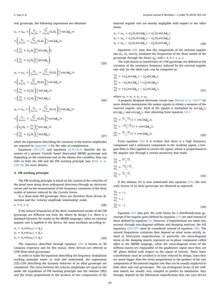
The first three real modes of the structure, which are designed to be
three ideal pure translational modes in the directions x, y and z, are
actually characterized by non-uniform displacement fields, s (see
Fig. 2b), that are here represented as:
=
⎡
⎣
⎢
⎢
⎤
⎦
⎥
⎥
= φx y z t
φ x y z u t
φ x y z u t
φ x y z u t
ts x u( , , , )
( , , ) ( )
( , , ) ( )
( , , ) ( )
( ) ( ),
x
x
y
y
z
z (9)
where φ x( ) is the diagonal matrix containing the three nondimensional
modal shape functions φx, φy, φz describing the three main modes
actuated by on board actuators in a real gyroscope (see Section 5) and
=t u t u t u tu ( ) [ ( ), ( ), ( )]T
x y z is the time evolution of the system's re-
sponse with ux, uy and uz the amplitudes of the three modes. Note that,
rotational degrees of freedom will not be included in the present for-
mulation. This simplification is justified by the assumption that a
proper mechanical design would allow to obtain rotational modes at
very high frequencies with respect to those of the translational modes.
Denoting by ρ the density of the distributed mass with volume V, the
kinetic and potential energy of the real gyroscope read:
T
V V
∫= ⋅ = + + ∧ +
= ⋅ +
ρ Vv v v v s Ω s x
s x k s x
d with ˙ ( ),
( ) ( ) ,
V
eq ext
1
2 0 0
1
2 (10)
where keq is the non-diagonal equivalent stiffness matrix. The vector of
the generalized forces Q is constituted by the damping forces − b s x˙ ( )eq
with beq equivalent damping matrix that takes into account the fabri-
cation imperfections through extra-diagonal terms.
Neglecting again contributions coming from the external velocity
and acceleration, by substituting equation (10) into (2), the equations
of motion of a real three-axial gyroscope are derived. They read:
+ + + + + + +
+ + + + + + +
+ + + + +
α α α α
α α β β β β
β β β β β
mu bu ku u
u
u = F
¨ ˙ (Ω˙ ˆ Ω˙ ˆ Ω˙ ˆ ) 2(Ω ˆ
Ω ˆ Ω ˆ ) ˙ (Ω ˆ Ω ˆ Ω ˆ Ω Ω ( ˆ
ˆ ) Ω Ω ( ˆ ˆ ) Ω Ω ( ˆ ˆ ))
x
x
y
y
z
z
x
x
y
y
z
z
x
xx
y
yy
z
zz
x y
xy
yx
x z
xz zx
y z
yz zy
2 2 2
(11)
where, m is the diagonal mass matrix whose non-zero elements are the
modal masses of the three modes of interest, k is the stiffness matrix
that contains extra-diagonal terms coming from the fabrication im-
perfections, αˆi
and βˆij
, with =i j x y z, , , , are the coupling matrices that
arise because of the presence of the external angular velocities.
The matrices m, b and k have components mhk, bhk and khk re-
spectively with h and k taking values x, y and z. The terms of the ma-
trices m, b, k, αˆ and βˆ are defined as:
∫
∫
∫
= =
= =
= =
= − =
= − =
m ρφ φ δ V h k x y z
b φ b φ h k x y z
k φ k φ h k x y z
α ρε φ φ V i h k x y z
β ρ φ φ δ δ δ δ φ V i j h k x y z
x x
x x
d , , ,
( )( ) ( ) , , ,
( )( ) ( ) , , ,
ˆ d , , , ,
ˆ ( ( ) )d , , , , ,
hk
V
h k
hk
hk
h
eq hk
k
hk
h
eq hk
k
hk
i
V
ihk
h k
hk
ij
V
h k
ih jk ij hk
h 2
(12)
where the summation over repeated indices is not considered.
The angular gain αhk
i
with =i h k x y z, , , , of the distributed-mass
gyroscope is defined as the ratio between αˆhk
i
and the modal mass mhh
as:
= − =α
α
m
i h k x y z
ˆ
(distributed mass) , , , , .hk
i hk
i
hh (13)
Note that in the limit of pointwise mass →φ 1h , →m mhh and
equation (13) coincides with equation (5). In general, since φh vary in
space, the entries of the angular gain matrices αi
differ from unit.
Finally, note that the external velocities and accelerations can be
neglected even when the external acceleration is not negligible; it is
possible in fact to null their contributions through the design of a dif-
ferential mechanical structure as shown in Zega et al. (2017b).
3. Phasor analysis
The equations of motion presented in the previous section are, here,
solved through the phasor method (see Kline et al. (2013b)) both for the
case of an ideal point-mass gyroscope and for a real gyroscope.
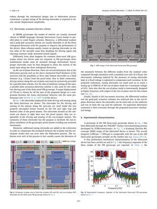
V. Zega et al. European Journal of Mechanics / A Solids 70 (2018) 203–212
205

4. 3.1. Ideal gyroscope
Accounting for relations (5)–(6), the vectorial equation (4) can be
written in the scalar form:
+ − + + − + +
+ − + + =
+ − + + − + +
+ + + − =
+ − + + − + +
+ − + + =
mx b x m y m z k x m x
m y m z F
my b y m z m x k y m y
m x m z F
mz b z m x m y k z m z
m x m y F
¨ ˙ 2 Ω ˙ 2 Ω ˙ (Ω Ω )
(Ω Ω Ω˙ ) (Ω˙ Ω Ω ) ,
¨ ˙ 2 Ω ˙ 2 Ω ˙ (Ω Ω )
(Ω Ω Ω˙ ) (Ω Ω Ω˙ ) ,
¨ ˙ 2 Ω ˙ 2 Ω ˙ (Ω Ω )
(Ω Ω Ω˙ ) (Ω˙ Ω Ω ) .
x z y x z y
x y z y x z x
y x z y z x
x y z z y x y
z y x z x y
x z y x y z z
2 2
2 2
2 2
(14)
In order to make clearer the link between the results for the ideal
gyroscope and those for a real one, we keep here the notation with αhk
i
and βhk
ij
, without substituting their values given in (5)–(6). Equation
(14) will hence be written in the form:
⎜ ⎟
⎜ ⎟
⎜ ⎟ ⎜ ⎟
⎜ ⎟
+ + + + + + +
+ ⎛
⎝
+ ⎞
⎠
+ + =
+ + + + + ⎛
⎝
+ ⎞
⎠
+
+ ⎛
⎝
+ ⎞
⎠
+ ⎛
⎝
+ ⎞
⎠
=
+ + + + + + +
+ + + ⎛
⎝
+ ⎞
⎠
=
mx b x mα y mα z k x m β β x
m β α y m β α z F
my b y mα z mα x k y m β β y
m β α x m β α z F
mz b z mα x mα y k z m β β z
m β α x m β α y F
¨ ˙ 2 Ω ˙ 2 Ω ˙ ( Ω Ω )
Ω Ω Ω˙ ( Ω Ω Ω˙ ) ,
¨ ˙ 2 Ω ˙ 2 Ω ˙ Ω Ω
Ω Ω Ω˙ Ω Ω Ω˙ ,
¨ ˙ 2 Ω ˙ 2 Ω ˙ ( Ω Ω )
( Ω Ω Ω˙ ) Ω Ω Ω˙ ,
x xy
z
z xz
y
y x x
z
z x
y
y
xy
xy
x y xy
z
z xz
xz
x z xz
y
y x
y yz
x
x yx
z
z y y
z
z y
x
x
yx
yx
x y yx
z
z yz
yz
z y yz
x
x y
z zx
y
y zy
x
x z z
x
x z
y
y
zx
zx
x z zx
y
y zy
zy
y z zy
x
x z
2 2
2 2
2 2
(15)
where the double identical index has been substituted by a single one
for the sake of clarity.
In order to compensate for losses and to sustain the oscillation of the
gyroscope proof mass according to the three translational modes of
interest, the excitation forces can be written in the form
= F e F e F eF [(i ) , (i ) , (i ) ]T
x
ϕ
y
ϕ
zs
ϕi i ix y z with i imaginary unit, since at re-
sonance, the force needed to sustain the oscillation is in quadrature
with the displacement. Moreover, in the control circuit, the phase of the
forcers are derived directly from the phase of the gyroscope output, so it
is possible to say that, supposing a high quality factor Q for all the three
resonators, the complex solution of (15) can be constituted by three
sinusoidal oscillations near to the mechanical resonant frequency of
each axis, of the form:
⎡
⎣
⎢
⎤
⎦
⎥=
⎡
⎣
⎢
⎢
⎤
⎦
⎥
⎥
=u
u
u
u
A e
A e
A e
,
x
y
z
x
ϕ
y
ϕ
z
ϕ
i
i
i
x
y
z
(16)
where Ax, Ay, Az, ∫=ϕ ω τ τ( )dx
t
x0
, ∫=ϕ ω τ τ( )dy
t
y0
and ∫=ϕ ω τ τ( )dz
t
z0
represent the system unknowns. Ax, Ay, Az are the real, time dependent
amplitudes of the displacements of the proof mass along the three di-
rections x y, and z, while ω ω,x y and ωz are the actual resonant fre-
quencies of the three translational modes along the − −x y, and z-di-
rections. If no external angular rate is applied, =ω ωi oi with ωoi natural
frequency of the −i mode and = +ϕ ω t ψi oi i. In the following we in-
troduce the notation = −ϕ ϕ ϕΔ ij i j with =i x y z, , .
Note that Ax, Ay, Az, ωx, ωy and ωz are slowly varying relatively to
the mechanical resonant frequencies of the system, as a consequence, in
the acceleration expression, the terms containing A¨x, A¨y, A¨z, ω˙ x, ω˙ y and
ω˙ z can be neglected, as they are negligible if compared to ω A˙x x, ω A˙y y,
ω A˙z z, ωx
2
, ωy
2
and ωz
2
, respectively. Moreover, it is reasonable to assume
that the angular rate and the displacement amplitudes are slowly
varying with respect to the resonance frequency.
Under these hypotheses, by substituting equation (16) into (15) and
dividing the three equations for e ϕi x, e ϕi y and e ϕi z respectively, three
complex equations are obtained. By nulling both the real and the
imaginary parts, it is possible to obtain an expression for A˙x, A˙y, A˙ z, ωx
2
,
ωy
2
and ωz
2
.
The expressions for A˙x, A˙y and A˙ z are reported in Appendix A since
they will not be used in the following, while the expressions for ωx
2
, ωy
2
and ωz
2
under the assumption ≪A A ω˙ i i i for =i x y z, , read:
= + + +
+ + +
+ +
ω ω β β
β ϕ β ϕ
α ω ϕ α ω ϕ
Ω Ω
Ω Ω cos(Δ ) Ω Ω cos(Δ )
2 Ω sin(Δ ) 2 Ω sin(Δ ),
x ox x
z
z x
y
y
xy
xy
x y
A
A xy xz
xz
x z
A
A xz
xy
z
z y
A
A xy xz
y
y z
A
A xz
2 2 2 2
y
x
z
x
y
x
z
x (17)
= + + +
+ + +
− +
ω ω β β
β ϕ β ϕ
α ω ϕ α ω ϕ
Ω Ω
Ω Ω cos(Δ ) Ω Ω cos(Δ )
2 Ω sin(Δ ) 2 Ω sin(Δ ),
y oy y
x
x y
z
z
yx
yx
x y
A
A xy yz
yz
y z
A
A yz
yx
z
z x
A
A xy yz
x
x z
A
A yz
2 2 2 2
x
y
z
y
x
y
z
y (18)
= + + +
+ + +
− −
ω ω β β
β ϕ β ϕ
α ω ϕ α ω ϕ
Ω Ω
Ω Ω cos(Δ ) Ω Ω cos(Δ )
2 Ω sin(Δ ) 2 Ω sin(Δ ).
z oz z
x
x z
y
y
zy
zy
y z
A
A yz zx
zx
x z
A
A xz
zx
y
y x
A
A xz zy
x
x y
A
A yz
2 2 2 2
y
z
x
z
x
z
y
z (19)
By defining the velocity amplitudes as =v A ωi i i for =i x y z, , and
solving the second order equation (17) with respect to ωx, the following
expression is found:
= +
+ + +
+ + +
ω ϕ
ϕ α ϕ
α ϕ ω D
Ω Ω cos(Δ )
Ω Ω cos(Δ ) Ω sin(Δ )
Ω sin(Δ ) ,
x
β
ω x y
v
v xy
β
ω x z
v
v xz xy
z
z
v
v xy
xz
y
y
v
v xz ox x
2
2
2
xy
xy
oy
y
x
xz
xz
oz
z
x
y
x
z
x (20)
where
⎜ ⎜ ⎟
⎟
= + + ⎛
⎝
⎛
⎝
⎞
⎠
+
+ + +
+ ⎞
⎠
D β β ϕ
ϕ α ϕ
α ϕ
Ω Ω Ω Ω cos Δ
Ω Ω cos(Δ ) Ω sin(Δ )
Ω sin(Δ ) .
x x
z
z x
y
y
β
ω x y
v
v xy
β
ω x z
v
v xz xy
z
z
v
v xy
y
y
v
v
2 2
2
2
xz xz
2
xy
xy
oy
y
x
xz
xz
oz
z
x
y
x
z
x
(21)
By proceeding in the same way for the other two axes and by noting
that ≫ω Doi i
2
for =i x y z, , , the instantaneous frequencies of oscillation
along the x-, y- and z-axis are derived:
= + +
+ +
+ +
ω ω ϕ
ϕ
α ϕ α ϕ
Ω Ω cos(Δ )
Ω Ω cos(Δ )
Ω sin(Δ ) Ω sin(Δ ),
x ox
β
ω x y
v
v xy
β
ω x z
v
v xz
xy
z
z
v
v xy xz
y
y
v
v xz
2
2
xy
xy
oy
y
x
xz
xz
oz
z
x
y
x
z
x (22)
= + +
+ +
+ −
ω ω ϕ
ϕ
α ϕ α ϕ
Ω Ω cos(Δ )
Ω Ω cos(Δ )
Ω sin(Δ ) Ω sin(Δ ),
y oy
β
ω x y
v
v xy
β
ω y z
v
v yz
yz
x
x
v
v yz yx
z
z
v
v xy
2
2
yx
yx
ox
x
y
yz
yz
oz
z
y
z
y
x
y (23)
= + +
+ +
− −
ω ω ϕ
ϕ
α ϕ α ϕ
Ω Ω cos(Δ )
Ω Ω cos(Δ )
Ω sin(Δ ) Ω sin(Δ ).
z oz
β
ω x z
v
v xz
β
ω y z
v
v yz
zx
y
y
v
v xz zy
x
x
v
v yz
2
2
zx
zx
ox
x
z
zy
zy
oy
y
z
x
z
y
z (24)
3.2. Real gyroscope
By applying the same procedure to the equation of motion (11) of a
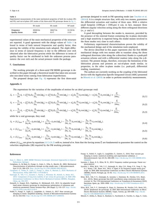
V. Zega et al. European Journal of Mechanics / A Solids 70 (2018) 203–212
206

5. real gyroscope, the following expressions are obtained:
⎟
⎟
⎜ ⎟
⎜ ⎟
= + ⎛
⎝
+ ⎞
⎠
+
+ ⎛
⎝
+ ⎞
⎠
+
+ + ⎞
⎠
+
+ + ⎞
⎠
( )
( )
ω ω ϕ
ϕ
α ϕ
α ϕ
Ω Ω cos(Δ )
Ω Ω cos(Δ )
Ω sin(Δ
Ω sin(Δ ,
x ox
k
ω m
β
ω m x y
v
v xy
k
ω m
β
ω m x z
v
v xz
b
m xy
z
z
v
v xy
b
m xz
y
y
v
v xz
2
ˆ
2
2
ˆ
2
2
2
xy
oy x
xy
xy
oy x
y
x
xz
oz x
xz
xz
oz x
z
x
xy
x
y
x
xz
x
z
x
(25)
⎜ ⎟
⎜ ⎟
= + ⎛
⎝
+ ⎞
⎠
+
+ ⎛
⎝
+ ⎞
⎠
+
+ + +
− +
( )
( )
ω ω ϕ
ϕ
α ϕ
α ϕ
Ω Ω cos(Δ )
Ω Ω cos(Δ )
Ω sin(Δ )
Ω sin(Δ ),
y oy
k
ω m
β
m ω x y
v
v xy
k
ω m
β
m ω y z
v
v yz
b
m yz
x
x
v
v yz
b
m yx
z
z
v
v xy
2
ˆ
2
2
ˆ
2
2
2
yx
ox y
yx
yx
y ox
x
y
yz
oz y
yz
yz
y oz
z
y
yz
y
z
y
xy
y
x
y (26)
⎜ ⎟
⎜ ⎟= + ⎛
⎝
+ ⎞
⎠
+
+ ⎛
⎝
+ ⎞
⎠
+
− + +
− +
( )
( )
ω ω ϕ
ϕ
α ϕ
α ϕ
Ω Ω cos(Δ )
Ω Ω cos(Δ )
Ω sin(Δ )
Ω sin(Δ ),
z oz
k
ω m
β
m ω x z
v
v xz
k
ω m
β
m ω y z
v
v yz
zx
y
y
b
m
v
v xz
b
m zy
x
x
v
v yz
2
ˆ
2
2
ˆ
2
2
2
zx
ox z
zx
zx
z ox
x
z
yz
oy z
zy
zy
z oy
y
z
xz
z
x
z
yz
z
y
z (27)
while the expressions describing the variation of the motion amplitudes
are reported in Appendix A for the sake of completeness.
Equations (25)-(27) and equations (A.4)-(A.6) describe the dy-
namics of a generic Coriolis based three-axial MEMS gyroscope and
depending on the constraints and on the chosen free variables, they can
refer to both the AM and the FM working principle (see Kline et al.
(2013b) for more details).
4. FM working principle
The FM working principle is based on the control of the velocities of
the proof mass along three orthogonal directions through an electronic
circuit and on the measurement of the frequency variations of the three
modes of interest induced by the Coriolis forces.
In a three-axial FM gyroscope, there are therefore three driven di-
rections and the ’velocity amplitude relationship’ reads:
= =v v v .x y z (28)
If the natural frequencies of the three translational modes of the FM
gyroscope are different one from the others by design (i.e. there is a
mismatch between the modes in the MEMS language), when no external
angular rate is applied to the device, the mass oscillates according to:
= +
= +
= +
u A ω t ψ
u A ω t ψ
u A ω t ψ
cos( ),
cos( ),
cos( ).
x x ox x
y y oy y
z z oz z (29)
The trajectory described through equation (29) is known as 3D
Lissajous trajectory and for this reason, these devices are referred as
LFM three-axial gyroscopes.
In order to make the equations describing the frequency modulation
working principle easier to read and understand, the expressions
(22)–(24) describing the dynamic behavior of an ideal gyroscope are
considered. The ratios between the velocity amplitudes are equal to one
under the hypothesis of FM working principle (see the relation (28))
and the terms proportional to the product of two components of the
external angular rate are usually negligible with respect to the other
terms:
= + +
= + −
= − −
ω ω α ϕ α ϕ
ω ω α ϕ α ϕ
ω ω α ϕ α ϕ
Ω sin(Δ ) Ω sin(Δ ),
Ω sin(Δ ) Ω sin(Δ ),
Ω sin(Δ ) Ω sin(Δ ).
x ox xy
z
z xy xz
y
y xz
y oy yz
x
x yz yx
z
z xy
z oz zx
y
y xz zy
x
x yz (30)
Equations (30) state that the components of the external angular
rate Ωx, Ωy and Ωz modulate the frequencies of the three modes of the
gyroscope through the factor αhk
i
with =i h k x y z, , , , .
The scale factors or sensitivities of a FM gyroscope are defined as the
variation of the resonance frequency induced by the external angular
rate and, for the ideal case, can be computed as:
= + −
= − +
= + −
∂
∂
∂
∂
∂
∂
α ϕ α ϕ
α ϕ α ϕ
α ϕ α ϕ
sin(Δ ) sin(Δ ),
sin(Δ ) sin(Δ ),
sin(Δ ) sin(Δ ),
ω
yz
x
yz zy
x
yz
ω
zx
y
xz xz
y
xz
ω
xy
z
xy yx
z
xy
Ω
Ω
Ω
x
y
z
Σ
Σ
Σ
(31)
where = + +ω ω ω ωx y zΣ .
A properly designed electronic circuit (see Minotti et al. (2017) for
more details) manipulates the output signals to obtain a measure of the
external angular rate. Each of the signals is multiplied by ϕsin(Δ )yz ,
ϕsin(Δ )xz and ϕsin(Δ )xy , thus obtaining from equation (31):
= +
= +
= +
∂
∂
−
∂
∂
− +
∂
∂
−
ϕ
ϕ
ϕ
(1 cos(2Δ )),
(1 cos(2Δ )),
(1 cos(2Δ )).
ω α α
yz
ω α α
xz
ω α α
xy
Ω 2
Ω 2
Ω 2
x
yz
x
zy
x
y
zx
y
xz
y
z
xy
z
yx
z
Σ
Σ
Σ
(32)
From equation (32) it is evident that there is a high frequency
component and a stationary component in the resultant signal, a low-
pass filter is then applied to extract the signal, which is proportional to
the angular rate through a certain sensitivity that reads:
=
=
=
∂
∂
−
∂
∂
− +
∂
∂
−
,
,
.
ω α α
ω α α
ω α α
Ω 2
Ω 2
Ω 2
x
yz
x
zy
x
y
zx
y
xz
y
z
xy
z
yx
z
Σ
Σ
Σ
(33)
If the relation (5) is now substituted into equation (33), the unit
scale factors of an ideal gyroscope are obtained as expected:
= −
=
= −
∂
∂
∂
∂
∂
∂
1,
1,
1.
ω
ω
ω
Ω
Ω
Ω
x
y
z
Σ
Σ
Σ
(34)
Equation (33) also give the scale factor for a distributed-mass gy-
roscope if the angular gains defined by equation (13) are used instead of
those defined by equation (5). However, if imperfections are taken into
account through non-diagonal stiffness and damping matrices, the full
equations (25)-(27) must be considered instead of equation (30). The
natural frequencies variations then depend on other terms strictly re-
lated to fabrication imperfections, in particular the extra-diagonal
terms of the damping matrix represent an in-phase component called
offset in the MEMS language, while the extra-diagonal terms of the
stiffness matrix are responsible of the quadrature signal since they are
90° phase shifted with respect to the signal of interest. These latter
contributions must be avoided or at least reduced by design, since they
are much bigger than the terms proportional to the product of the two
components of the external angular rate that can be usually neglected in
both ideal and real gyroscopes. The out-of-diagonal terms of the stiff-
ness matrix are usually very complex to predict by simulation: they
strongly depend on the fabrication imperfections that can vary device
V. Zega et al. European Journal of Mechanics / A Solids 70 (2018) 203–212
207

6. by device and run by run. It is in principle possible to estimate how
fabrication imperfections (e.g. over etch non-uniformity, eigenstrain)
affect the out-of-diagonal elements through statistical methods
(Mirzazadeh et al., 2017).
Summarizing, in order to implement a real three-axial FM gyro-
scope, it is necessary to minimize by design the non-ideal terms (e.g.
through the maximization of the decoupling between the three modes)
and to have a proper algorithm for the detection of the output signal
able to distinguish between offset, quadrature and the wanted signal
(see Minotti et al. (2018) for more details on the electronic circuit).
Once the electronic circuit identifies the signal of interest, the expres-
sion of the scale factors of a real three-axial FM gyroscope is the same as
(32) where αhk
i
with =i h k x y z, , , , are the angular gains defined
through equation (13). They depend only on geometrical quantities
being strictly related to the mass distribution of the mechanical struc-
ture and on the coupling among the modes. For this reason, the scale
factors of a three-axial FM gyroscope are little dependent on over etch
and other fabrication imperfections and are completely independent
from environmental fluctuations such as temperature. This property
represents the main advantage of the FM gyroscope with respect to the
AM counterpart.
5. Mechanical design
The proof mass of a three-axial FM gyroscope must be able to si-
multaneously translate along the three orthogonal directions. Proper
deformable portions and auxiliary structures must, then, be designed in
order to guarantee the wanted motion of the gyroscope's proof mass and
a good decoupling between the three modes of interest. In order to
reject the effect of inertia forces possibly coming from an external ac-
celeration and for a better functioning of the gyroscope as explained in
Section 5.2, a fully differential two-masses structure is here proposed.
The introduction of a second mass actuated in an antiphase mode in
the mechanical structure of the three-axial gyroscope allows the re-
jection of any unwanted common-mode contribution due e.g. to the
external acceleration (see Zega et al. (2017b) for more details).
In Fig. 3, a schematic and simplified view of the three modes of a FM
three-axial gyroscope compatible with the surface micromachining
fabrication process is shown. Note that surface micromachining pro-
cesses do not allow the exploitation of fully three-dimensional me-
chanical designs: in-plane structures are in fact extruded in the z-di-
rection and consequently a uniform out-of-plane thickness, with a value
fixed by the technological process, must be considered. The mechanical
structure must then be properly designed to overcome such strict lim-
itation of the fabrication process especially for the out-of-plane modes.
In this paper we show an innovative mechanical design that fullfils
all the requirements of the FM working principle and respects the
fabrication process constraints. In Fig. 3, a schematic view of the pro-
posed structure is shown. The two suspended proof masses (colored in
blue in Fig. 3) have three degrees of freedom as whished, while the
external frames have only one degree of freedom (indicated by the pink
arrows in Fig. 3) to allow for a good decoupling between the modes.
A central cross-shaped auxiliary structure is added to allow the anti-
phase motion of the two proof masses along the three orthogonal di-
rections. The deformation of the springs connecting the central struc-
ture to the two proof masses allows the differential x-mode (see Fig. 3a)
while the in-plane rotation of the horizontal central bridge (see Fig. 3b)
allows the differential y-mode. Finally, the out-of-plane torsional mo-
tion of the full cross-shaped auxiliary mass allows the differential z-
mode (see Fig. 3c). The black squares in Fig. 3 represent the anchors to
the substrate. In surface micromachining processes, in fact, the struc-
tures are suspended through springs and are at a fixed distance from the
substrate. As it will be clearer later, this is another constraint that the
MEMS designer must take into account during the design process.
5.1. Implementation of the three-axial FM gyroscope
Starting from the schematic view shown in Fig. 3, a real design of a
three-axial FM gyroscope compatible with the Thelma©
surface mi-
cromachining process of STMicroelectronics (see Corigliano et al.
(2004) for more details) has been studied.
In Fig. 4, an in-plane view of the mechanical design of the proposed
three-axial FM gyroscope is represented: it is possible to recognize the
two proof masses, the external frames and the central cross-shaped
auxiliary structure composed by two torsional masses and a central
bridge. Fig. 5 shows the shapes of the three anti-phase translational
modes of the gyroscope's structure.
The central bridge that can rotate around the out-of-plane z-axis
with respect to the torsional masses thanks to the two hinge-like con-
nections (see Fig. 4), allows the differential motion of the proof masses
of the gyroscope along the y-axis direction (see Fig. 5a). Note that
hinge-like connections must be obtained through short thin beams since
it is not possible to obtain such kind of connections in standard MEMS
fabrication processes.
The springs connecting the central bridge with the proof masses are
mainly responsible of the anti-phase motion of the masses along the x-
axis (see Fig. 5b).
The two auxiliary torsional masses are anchored to the substrate
Fig. 3. Schematic view of the three-axial FM gyroscope. Differential mode along the (a) x-
axis, (b) y-axis and (c) z-axis.
V. Zega et al. European Journal of Mechanics / A Solids 70 (2018) 203–212
208

7. through torsional springs (two elongated beams located in the middle of
the torsional masses and one folded spring sited on top (bottom) of the
mass as shown in Fig. 4e–f) that allow their rotation around the y-axis
thus coupling, in a differential way, the two proof masses of the gyro-
scope during the out-of-plane mode (see Fig. 5c). The out-of-plane
translational motion of the proof masses is then achieved thus over-
coming one of the major constraint of the surface micromachining
process. Thanks to this shrewdness, in fact, we obtain an innovative
mechanical structure able to translate in the z-direction: on the con-
trary, almost all the MEMS devices available so far exploit the torsional
modes for the out-of-plane driving/sensing.
From Fig. 5 one can observe that the proof masses of the three-axial
FM gyroscope are well decoupled from the external frames containing
the in-plane electrodes thanks to the ring-like springs shown in Fig. 4c
(see Zega et al. (2017b) for more details on the working principle of
such spring). The displacement of the x-axis (y-axis) external frames
during the y-mode (x-mode) is less than 1/10 (1/19) of the motion of
the proof masses while the displacement of the external frames during
the z-mode of the device is less than 1/30 of the out-of-plane motion of
the two proof masses. The suspending springs connecting the external
frames to the substrate (see Fig. 4b) allow only one degree of freedom
and consequently improve the decoupling between the modes.
In Table 1 the main mechanical properties computed though Finite
Element (FE) analyses for a standard over etch, are summarized. The
quality factor estimation is carried out through the numerical code
based on the Boundary Integral Equation approach presented in Frangi
et al. (2016) and Fedeli et al. (2017).
The modes have been designed such as to guarantee comparable
stiffness and modal mass for the three axes. Despite the fabrication
process forces a completely different geometry in-plane and out-of-
plane, a proper design of the springs and the masses allows to obtain
similar mechanical properties for the three modes of interest. This is
fundamental in such devices where the scale factor only depends on the
modal masses involved in the modes. The expected sensitivity can be
calculated from equations (33) and (13) and is equal to 0.92, 0.91 and
0.84 for x, y and z respectively.
The difference in terms of quality factor is actually very difficult to
Fig. 4. Schematic in-plane view of the three-axial FM gyroscope.
Fig. 5. Modal analysis of the three-axial FM gyroscope performed in
COMSOLMultiphysics©
. The contour of the magnitude of the displacement field is shown
in color. Only the three differential translational modes of interest are shown: a) y-axis
mode ( =f 44087 Hz), b) x-axis mode ( =f 44150 Hz), c) z-axis mode ( =f 45712 Hz). (For
interpretation of the references to color in this figure legend, the reader is referred to the
Web version of this article.)
Table 1
Main mechanical properties of both the in-plane (IPx and IPy) and out-of-plane (OP)
modes of the three-axial FM gyroscope shown in Fig. 4.
IPx mode IPy mode OP mode
Frequency 44150 Hz 44087 Hz 45712 Hz
Stiffness 3295 N/m 3127 N/m 2921 N/m
Modal Mass 39 nKg 38 nKg 33 nKg
Quality factor 7000 7500 950
V. Zega et al. European Journal of Mechanics / A Solids 70 (2018) 203–212
209

8. reduce through the mechanical design, due to fabrication process
constraints: a proper sizing of the driving electrodes is required to ob-
tain similar displacement amplitudes.
5.2. Electrostatic actuation/detection schemes
In MEMS gyroscopes the modes of interest are usually actuated
(driven in MEMS language) through electrostatic forces thanks to par-
allel plate or comb fingers schemes. Moreover, a differential readout
and a push-pull actuation scheme are usually desirable in all the three
orthogonal directions with the purpose to improve the performance of
the device: these schemes mainly consist on placing electrodes on the
two sides of the movable mass thus doubling the driving signal and
rejecting common mode unwanted sensed signals.
Differently from what happens for common three-axial AM gyro-
scopes where two driven axes are required, in FM gyroscopes three
translational modes must be actuated through electrostatic forces:
proper electrodes must be then designed to allow the motion of the
proof mass along the three orthogonal directions.
In the out-of-plane direction, there are several limitations due to the
fabrication process such as the above mentioned fixed thickness of the
structure and the possibility to have only bottom electrodes at a fixed
distance (e.g. 1.8 μm) from the proof mass. Due to these constraints,
driving motion along the out-of-plane axis must be exclusively provided
by a parallel plate scheme. For the sake of similarity among all the axes,
a parallel plate actuation/detection scheme is also used for the other
two driving axes of the three-axial FM gyroscope. A target displacement
of 170 nm is chosen for all the axes of the proposed design as a com-
promise between the linear electrostatic behavior and the noise per-
formance (see Minotti et al. (2017)) of the device.
In Fig. 6 the electrodes employed for both driving and sensing along
the three directions are shown. The electrodes for the driving and
sensing of the motion along the x(y)-axis are sited inside the two
properly decoupled frames located on the left and right (top and
bottom) sides of the proof masses. The electrodes located on the sub-
strate are shown in light blue over the proof masses: they are re-
sponsible of the driving and sensing of the out-of-plane motion. The
symmetry of these electrodes has the purpose to facilitate the out-of-
plane translation of the gyroscope's proof masses avoiding any torsional
movements.
Moreover, additional tuning electrodes are added in the z-direction
in order to compensate the mismatch between the in-plane and the out-
of-plane modes that can arise after the fabrication process. The un-
known over etch of the process in fact usually causes the deviation of
the mismatch between the different modes from the nominal value
computed through simulation with a standard over etch of 0.35 μm: the
electrostatic softening induced by the presence of tuning electrodes
kept at a fixed voltage is exploited to compensate such variation. In the
proposed realization, tuning electrodes are sized such as to reach a
tuning up to 2000 Hz of the out-of-plane mode for a maximum voltage
of 23 V. Note also that the out-of-plane mode is intentionally designed
at higher frequency with respect to the two in-plane ones for this reason
(see Fig. 5).
Finally, thanks to the two-masses structure, the differential readout
and the push-pull actuation schemes are achieved also in the out-of-
plane direction where the electrodes can be sited only on the substrate
and not on both the cap and the substrate. An important fabrication
constraint is then overcame through the proposed innovative mechan-
ical design.
6. Experimental characterization
A prototype of the FM three-axial gyroscope shown in Fig. 4 has
been fabricated through the ThELMA©
surface micromachining process
developed by STMicroelectronics. In Fig. 7, a Scanning Electron Mi-
croscope (SEM) image of the fabricated device is shown. The overall
footprint (1089 μm × 1595 μm) is comparable with the one of the AM
three-axial gyroscopes actually on the market (see e.g. Vigna (2011)).
A first preliminary mechanical characterization of the fabricated
device has been carried out and in Fig. 8 the frequency responses of the
three modes of the FM gyroscope are reported. In Table 2, the
Fig. 6. Schematic in-plane view of both the in-plane (IPx and IPy) and out-of-plane (OP)
electrodes for the three-axial FM gyroscope shown in Fig. 4.
Fig. 7. SEM image of the fabricated three-axial FM gyroscope.
Fig. 8. Experimental frequency response of the fabricated three-axial FM gyroscope
shown in Fig. 7.
V. Zega et al. European Journal of Mechanics / A Solids 70 (2018) 203–212
210

9. experimental values of the main mechanical properties of the structure
are reported. A good agreement with the design values of Table 1 is
found in terms of both natural frequencies and quality factor, thus
proving the validity of the simulation tools adopted. The slight differ-
ence in terms of natural frequency is due to the different over etch
obtained after the fabrication process while the difference in terms of
quality factor can be attributed to both the unknown process para-
meters: the over etch and the actual pressure inside the package.
7. Conclusions
The working principle of a three-axial FM MEMS gyroscope is de-
scribed in this paper through a theoretical model that takes into account
also non-ideal terms coming from fabrication imperfections.
The proposed design (see Fig. 4) represents the first three-axial
gyroscope designed to work in FM operating mode (see Tocchio et al.
(2016)). It is a simple structure that, with only two masses, guarantees
the differential actuation and readout of three axes. With a relative
small footprint (1090 μm × 1595 μm) it can, in fact, measure three
different angular velocities acting along the three orthogonal directions
(x-, y- and z-).
A good decoupling between the modes is, moreover, provided by
the presence of the external frames containing the in-plane electrodes
and a high sensitivity is expected being the modal masses involved in
the three modes very close to each others.
Preliminary experimental characterizations proves the validity of
the mechanical design and of the simulation tools employed.
The device described in this paper represents also the first MEMS
mechanical design with two masses able to translate along the three
orthogonal directions (also along the z-direction) thanks to a push-pull
actuation scheme and with a differential readout (also along the z-di-
rection). The present design, therefore, overcame the limitations of the
fabrication process and presents an out-of-plane mode similar, in
properties, to the other in-plane modes (i.e. push-pull, differential
reading, translation).
The authors are currently working on the coupling of the fabricated
device with the Application Specific Integrated Circuit (ASIC) presented
in Minotti et al. (2018) in order to perform sensitivity measurements.
Appendix A
The expressions for the variation of the amplitudes of motion for an ideal gyroscope read:
= − + + − − +A
b
m
A β
A
ω
ϕ β
A
ω
ϕ α
ω
ω
A ϕ α
ω
ω
A ϕ
F
mω
˙
2
Ω Ω
2
sin(Δ ) Ω Ω
2
sin(Δ ) Ω cos(Δ ) Ω cos(Δ )
2
,x
x
x xy
xy
x y
y
x
xy xz
xz
x z
z
x
xz xy
z
z
y
x
y xy xz
y
y
z
x
z xz
x
x (A.1)
= − − + − − +A
b
m
A β
A
ω
ϕ β
A
ω
ϕ α
ω
ω
A ϕ α
ω
ω
A ϕ
F
mω
˙
2
Ω Ω
2
sin(Δ ) Ω Ω
2
sin(Δ ) Ω cos(Δ ) Ω cos(Δ )
2
,y
y
y yx
yx
x y
x
y
xy yz
yz
y z
z
y
yz yx
z
z
x
y
x xy yz
x
x
z
y
z yz
y
y (A.2)
= − − − − − +A
b
m
A β
A
ω
ϕ β
A
ω
ϕ α
ω
ω
A ϕ α
ω
ω
A ϕ
F
mω
˙
2
Ω Ω
2
sin(Δ ) Ω Ω
2
sin(Δ ) Ω cos(Δ ) Ω cos(Δ )
2
,z
z
z zx
zx
x z
x
z
xz zy
zy
y z
y
z
yz zx
y
y
x
z
x xz zy
x
x
y
z
y yz
z
z (A.3)
while for a real gyroscope, they read:
= + + − −A A
k
ω m
A ϕ
k
ω m
A ϕ
b
m
ω
ω
A ϕ
b
m
ω
ω
A ϕ˙ ( ˙ )
2
sin(Δ )
2
sin(Δ )
2
cos(Δ )
2
cos(Δ ),x x ideal
xy
x x
y xy
xz
x x
z xz
xy
x
y
x
y xy
xz
x
z
x
z xz
(A.4)
= − + − −A A
k
ω m
A ϕ
k
ω m
A ϕ
b
m
ω
ω
A ϕ
b
m
ω
ω
A ϕ˙ ( ˙ )
2
sin(Δ )
2
sin(Δ )
2
cos(Δ )
2
cos(Δ ),y y ideal
yx
y y
x xy
yz
y y
z yz
yx
y
x
y
x xy
yz
y
z
y
z yz
(A.5)
= − − − −A A
k
ω m
A ϕ
k
ω m
A ϕ
b
m
ω
ω
A ϕ
b
m
ω
ω
A ϕ˙ ( ˙ )
2
sin(Δ )
2
sin(Δ )
2
cos(Δ )
2
cos(Δ ),z z ideal
zy
z z
y yz
zx
z z
x xz
zx
z
x
z
x xz
zy
z
y
z
y yz
(A.6)
where A( ˙ )i ideal are given by equations (A.1)-(A.3) with mi instead of m. Note that the forcing terms Fi are fundamental to guarantee the control on the
velocities amplitudes (28) required by the FM working principle.
References
Acar, C., Shkel, A., 2009. MEMS Vibratory Gyroscopes. Structural Approaches to Improve
Robustness. Springer.
Corigliano, A., De Masi, B., Frangi, A., Comi, C., Villa, A., Marchi, M., 2004. Mechanical
characterization of polysilicon through on-chip tensile tests. J. Microelectromech.
Syst 13 (2), 200–219. http://dx.doi.org/10.1109/JMEMS.2003.823221.
Corigliano, A., Ardito, R., Comi, C., Frangi, A., Ghisi, A., Mariani, S., 2018. Mechanics of
Microsystems. Wiley ISBN 978-1-119-05383-5.
Eminoglu, B., Yeh, Y.-C., Izyumin, I., Nacita, I., Wireman, M., Reinelt, A., Boser, B.E.,
2016. Comparison of long-term stability of am versus fm gyroscopes. In: IEEE 29th
International Conference on Micro Electro Mechanical Systems (MEMS), Shanghai,
China, pp. 954–957.
Esmaeili, A., Kupaei, M.A., Faghihian, H., Mirdamadi, H.R., 2014. An adaptable broad-
band mems vibratory gyroscope by simultaneous optimization of robustness and
sensitivity parameters. Sensor Actuator Phys. 206 (Suppl. C), 132–137. http://dx.doi.
org/10.1016/j.sna.2013.12.014.
Fedeli, P., Frangi, A., Laghi, G., Langfelder, G., Gattere, G., 2017. Near vacuum gas
damping in mems: simplified modeling. Journal of Microelectromechanical Systems
26 (3), 632–642. http://dx.doi.org/10.1109/JMEMS.2017.2686650.
Frangi, A., Fedeli, P., Laghi, G., Langfelder, G., Gattere, G., 2016. Near vacuum gas
damping in mems: numerical modeling and experimental validation. J.
Microelectromech. Syst 25 (5), 890–899. http://dx.doi.org/10.1109/JMEMS.2016.
2584699.
Izyumin, I., Boser, B. E., Kline, M. H., 2014. Frequency readout gyroscope. Patent wo/
2014/093727.
Izyumin, I., Kline, M.H., Yeh, Y.-C., Eminoglu, B., Ahn, C.H., Hong, V.A., Yang, Y., Ng,
E.J., Kenny, T.W., Boser, B.E., 2015. A 7ppm, 6°/hr frequency-output mems gyro-
scope. In: IEEE 28th International Conference on Micro Electro Mechanical Systems
(MEMS), Estoril, Portugal, pp. 33–36. http://dx.doi.org/10.1109/MEMSYS.2015.
7050879.
Kline, M.H., Yeh, Y.-C., Eminoglu, B., Izyumin, I., Daneman, M., Horsley, D.A., Boser,
B.E., 2013a. Mems gyroscope bias drift cancellation using continuous-time mode
reversal. In: The 17th International Conference on Transducers & Eurosensors XXVII,
Barcelona, Spain, pp. 1855–1858. http://dx.doi.org/10.1109/Transducers.2013.
6627152.
Kline, M.H., Yeh, Y.-C., Eminoglu, B., Najar, H., Daneman, M., Horsley, D.A., Boser, B.E.,
2013b. Quadrature fm gyroscope. In: IEEE 26th International Conference on Micro
Electro Mechanical Systems (MEMS), Taipei, Taiwan, pp. 604–608. http://dx.doi.
org/10.1109/MEMSYS2013.6474314.
Minotti, P., Dellea, S., Mussi, G., Bonfanti, A., Facchinetti, S., Tocchio, A., Zega, V., Comi,
Table 2
Experimental measurements of the main mechanical properties of both the in-plane (IPx
and IPy) and out-of-plane (OP) modes of the three-axial FM gyroscope shown in Fig. 4.
IPx mode IPy mode OP mode
Frequency 40528 Hz 40627 Hz 41150 Hz
Quality factor 6598 5117 1133
V. Zega et al. European Journal of Mechanics / A Solids 70 (2018) 203–212
211

10. C., Lacaita, A.L., Langfelder, G., 2018. High scale-factor stability frequency-modu-
lated mems gyroscope: 3-axis sensor and integrated electronics design. IEEE Trans.
Ind. Electron. 65 (6), 5040–5050. http://dx.doi.org/10.1109/TIE.2017.2772212.
Minotti, P., Mussi, G., Dellea, S., Comi, C., Zega, V., Facchinetti, S., Tocchio, A., Bonfanti,
A., Langfelder, G., 2017. A 160 μa, 8 mdps/hz1/2
frequency-modulated mems gyro-
scope. In: Inertial 2017, Kauai, Hawaii.
Mirzazadeh, R., Azam, S.E., Jansen, E., Mariani, S., 2017. Uncertainty quantification in
polysilicon mems through on-chip testing and reduced-order modelling. In: 2017
18th International Conference on Thermal, Mechanical and Multi-physics Simulation
and Experiments in Microelectronics and Microsystems (EuroSimE), pp. 1–8.
Sonmezoglu, S., Alper, S.E., Akin, T., 2014. An automatically mode-matched mems gy-
roscope with wide and tunable bandwidth. Journal of Microelectromechanical
Systems 23 (2), 284–297. http://dx.doi.org/10.1109/JMEMS.2014.2299234.
Sonmezoglu, S., Taheri-Tehrani, P., Valzasina, C., Falorni, L.G., Zerbini, S., Nitzan, S.,
Horsley, D.A., 2015. Single-structure micromachined three-axis gyroscope with re-
duced drive-force coupling. IEEE Electron. Device Lett. 36 (9), 953–956. http://dx.
doi.org/10.1109/LED.2015.2454511.
Taheri-Tehrani, P., Kline, M., Izyumin, I., Eminoglu, B., Yeh, Y.C., Yang, Y., Chen, Y.,
Flader, I., Ng, E.J., Kenny, T.W., Boser, B.E., Horsley, D.A., 2016. Epitaxially-en-
capsulated quad mass gyroscope with nonlinearity compensation. In: IEEE 29th
International Conference on Micro Electro Mechanical Systems (MEMS), pp.
966–969. http://dx.doi.org/10.1109/MEMSYS.2016.7421793.
Tatar, E., Alper, S.E., Akin, T., 2012. Quadrature-error compensation and corresponding
effects on the performance of fully decoupled mems gyroscopes. Journal of
Microelectromechanical Systems 21 (3), 656–667. http://dx.doi.org/10.1109/
JMEMS.2012.2189356.
Tatar, E., Mukherjee, T., Fedder, G.K., 2017. Stress effects and compensation of bias drift
in a mems vibratory-rate gyroscope. Journal of Microelectromechanical Systems 26
(3), 569–579. http://dx.doi.org/10.1109/JMEMS.2017.2675452.
Tocchio, A., Falorni, L., Comi, C., Zega, V., 2016. Giroscopio triassiale mems a mod-
ulazione di frequenza, deposited patent n.: 102016000106928.
Vigna, B., 2011. Tri-axial mems gyroscopes and six degree-of-freedom motion sensors. In:
IEEE International Electron Devices Meeting, Washington DC, USA, 29.1.1–3.
Wu, G., Chua, G., Gu, Y., 2017. A dual-mass fully decoupled mems gyroscope with wide
bandwidth and high linearity. Sensor Actuator Phys. 259, 50–56. http://dx.doi.org/
10.1016/j.sna.2017.03.027.
Zega, V., Minotti, P., Mussi, G., Tocchio, A., Falorni, L., Facchinetti, S., Bonfanti, A.,
Lacaita, A.L., Comi, C., Langfelder, G., Corigliano, A., 2017a. The first frequency
modulated (fm) pitch gyroscope. In: Proceedings 2017, Vol. 1, pp. 393.
Zega, V., Comi, C., Minotti, P., Falorni, L., Tocchio, A., Langfelder, G., Corigliano, A.,
2017b. Mechanical design of a fully-differential triaxial frequency modulated mems
gyroscope. In: AIMETA 2017-Proceedings of the XXIII Conference of the Italian
Association of Theoretical and Applied Mechanics, vol. 1. pp. 420–427.
V. Zega et al. European Journal of Mechanics / A Solids 70 (2018) 203–212
212