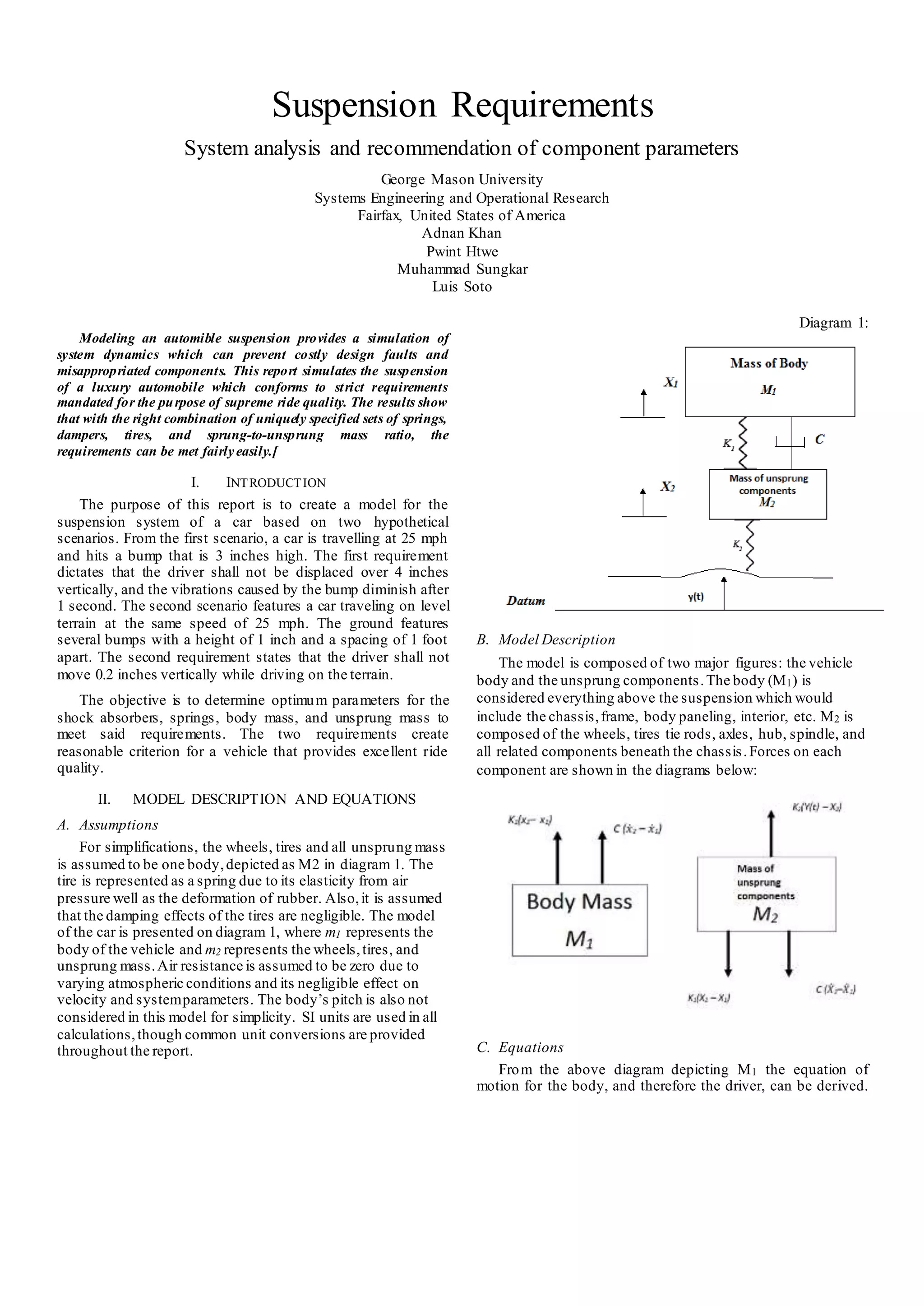
This document summarizes a student project that models the suspension system of a luxury automobile. The project aims to determine optimal parameters for springs, dampers, tires and masses to meet ride quality requirements. The model simulates two scenarios: 1) hitting a 3-inch bump at 25 mph and 2) traveling on bumpy terrain at 25 mph with 1-inch bumps spaced 1 foot apart. The results show that with the right component parameters, the requirements can be met. Parameters recommended are a 3000 kg body mass, 200 kg unsprung mass, 8 million N/m spring rate and 700,000 N*s/m damper constant.

1. Suspension Requirements
System analysis and recommendation of component parameters
George Mason University
Systems Engineering and Operational Research
Fairfax, United States of America
Adnan Khan
Pwint Htwe
Muhammad Sungkar
Luis Soto
Diagram 1:
Modeling an automible suspension provides a simulation of
system dynamics which can prevent costly design faults and
misappropriated components. This report simulates the suspension
of a luxury automobile which conforms to strict requirements
mandated for the purpose of supreme ride quality. The results show
that with the right combination of uniquely specified sets of springs,
dampers, tires, and sprung-to-unsprung mass ratio, the
requirements can be met fairlyeasily.[
I. INTRODUCTION
The purpose of this report is to create a model for the
suspension system of a car based on two hypothetical
scenarios. From the first scenario, a car is travelling at 25 mph
and hits a bump that is 3 inches high. The first requirement
dictates that the driver shall not be displaced over 4 inches
vertically, and the vibrations caused by the bump diminish after
1 second. The second scenario features a car traveling on level
terrain at the same speed of 25 mph. The ground features
several bumps with a height of 1 inch and a spacing of 1 foot
apart. The second requirement states that the driver shall not
move 0.2 inches vertically while driving on the terrain.
The objective is to determine optimum parameters for the
shock absorbers, springs, body mass, and unsprung mass to
meet said requirements. The two requirements create
reasonable criterion for a vehicle that provides excellent ride
quality.
II. MODEL DESCRIPTION AND EQUATIONS
A. Assumptions
For simplifications, the wheels, tires and all unsprung mass
is assumed to be one body,depicted as M2 in diagram 1. The
tire is represented as a spring due to its elasticity from air
pressure well as the deformation of rubber. Also,it is assumed
that the damping effects of the tires are negligible. The model
of the car is presented on diagram 1, where m1 represents the
body of the vehicle and m2 represents the wheels,tires, and
unsprung mass.Air resistance is assumed to be zero due to
varying atmospheric conditions and its negligible effect on
velocity and systemparameters. The body’s pitch is also not
considered in this model for simplicity. SI units are used in all
calculations,though common unit conversions are provided
throughout the report.
B. Model Description
The model is composed of two major figures: the vehicle
body and the unsprung components.The body (M1) is
considered everything above the suspension which would
include the chassis,frame, body paneling, interior, etc. M2 is
composed of the wheels, tires tie rods, axles, hub, spindle, and
all related components beneath the chassis.Forces on each
component are shown in the diagrams below:
C. Equations
From the above diagram depicting M1 the equation of
motion for the body, and therefore the driver, can be derived.

2. The following equation is related to ẍ1, the displacement of the
car’s body:
𝑥̈1 =
𝑘1 𝑥2 − 𝑘1 𝑥1 + 𝑐𝑥̇2 − 𝑐𝑥̇1
𝑚1
where 𝑘1 is the spring rate, 𝑥1 is the displacement of the
vehicle body, 𝑥2 is the movement of the tire, 𝑐 is the damping
constant ofthe shockabsorbers, 𝑥̇1 is the velocity of the car
body,and 𝑥̇2 is the velocity of the unsprung mass.
The equation for ẍ2, the acceleration of the unsprung
mass is:
𝑥̈2 =
𝑘2 𝑦 − 𝑘2 𝑥2 + 𝑘1 𝑥2 − 𝑐1 𝑥̇2 + 𝑐1 𝑥̇1
𝑚2
where y is the input force provided by the road in the form of
surface irregularities or bumps.
III. RESULTS
A. Tables and Figures
All tables and figures are included in the appendix to allow for
easier viewing. Please see refer to page 3 or section IV.
B. Analysis
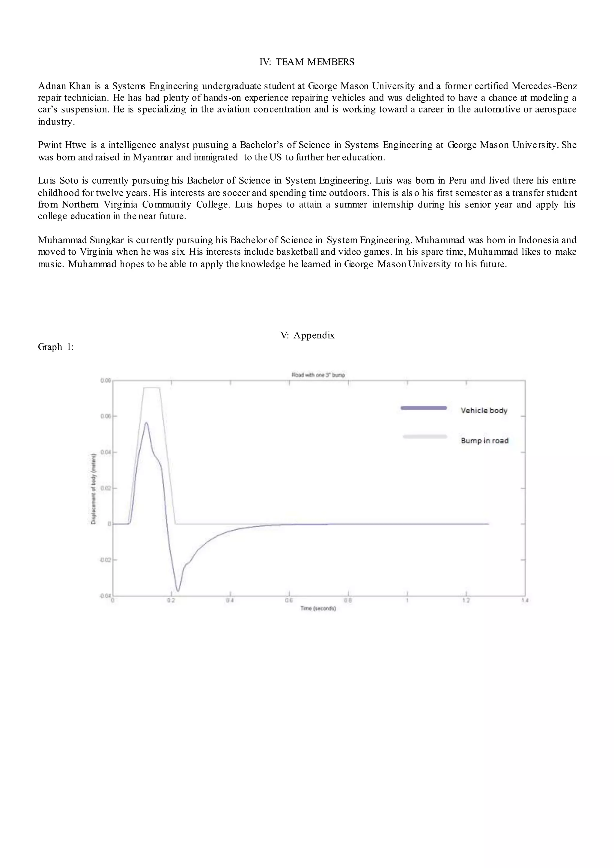
For the first scenario, the depicted graph (Appendix: graph
1) shows that the 0.076 meter (~3 inch) bump does not displace
the body more than approximately 0.05 meters, or 2 inches.
This value is well within the maximum allowable vertical
displacement of the driver, which is 4 inches.The shock
absorbers do well to reduce oscillation which is evident by the
systemstabilizing before the one-second mark on the x-axis,
meeting the requirement. However, the configuration may
prove to be too stiff; as the quick downward displacement of
the rigid body may prove to be uncomfortable for drivers. A
different shockand spring constant combination can likely
provide smoother transitions as the vehicle hits the bump and
clears it. The result also suggests that the two requirements
may not be a sufficient measure of ride quality.
From the graph 1 in the appendix, it appears that the input
force has a height of 4 inches and gradually decreases untilit
becomes a horizontal line. This result is plausible because the
amplitude corresponds to the displacement of the vertical. The
sine wave reaches a height of 0 on the one second mark, as
expected.
In the second scenario,the output graph (graph 2) is an
oscillating sine wave due to the evenly spaced bumps of equal
height.The systemmeets the second requirement as the body
does not deviate more than 0.0058 meters (0.2 inches).
Displacement appears to peak around -0.022 meters (0.08
inches)around the 0.2 seconds mark. Note that the
displacement of the body is lower than the height of the bump
due to the compression of the springs and dampers.
The recommendation for systemparameters acquired from
the two simulations is the following:
Mass ofbody: 3,000 kg
Mass ofwheels, tires, and suspension:200 kg
Spring rate: 8,000,000 N/m
Damper constant:700,000 N*s/m
CONCLUSION
The largest error in the system is likely the pitch of the
body which can have a considerable effect on suspension
behavior. Lumping all the unsprung mass into one mass is also
unpractical given that the springs and dampers are only
partially included in the unsprung mass. It is also difficult to
translate the large spring constant of the tire into air pressure,
and tire properties. All things considered, the system still
simulates a commonly used suspension configuration, and can
be used in the design process so long as the user is aware of the
assumptions.
References
[1] Palm III, William. System Dynamics.2nd
. New York: McGraw Hill,
2014.

3. IV: TEAM MEMBERS
Adnan Khan is a Systems Engineering undergraduate student at George Mason University and a former certified Mercedes-Benz
repair technician. He has had plenty of hands-on experience repairing vehicles and was delighted to have a chance at modeling a
car’s suspension. He is specializing in the aviation concentration and is working toward a career in the automotive or aerospace
industry.
Pwint Htwe is a intelligence analyst pursuing a Bachelor’s of Science in Systems Engineering at George Mason University. She
was born and raised in Myanmar and immigrated to the US to further her education.
Luis Soto is currently pursuing his Bachelor of Science in System Engineering. Luis was born in Peru and lived there his entire
childhood for twelve years. His interests are soccer and spending time outdoors. This is als o his first semester as a transfer student
from Northern Virginia Community College. Luis hopes to attain a summer internship during his senior year and apply his
college education in the near future.
Muhammad Sungkar is currently pursuing his Bachelor of Science in System Engineering. Muhammad was born in Indonesia and
moved to Virginia when he was six. His interests include basketball and video games. In his spare time, Muhammad likes to make
music. Muhammad hopes to be able to apply the knowledge he learned in George Mason University to his future.
V: Appendix
Graph 1:

4. Graph 2:
Matlab commands:
m1 = 3000; %kg
m2 = 200; %kg
k1 = 8000000; %Newtons per meter (N/m)
k2 = 80000000; %tire has a very high spring constant unit: N/m
c = 700000; %N*s /m
A = [0 1 0 0; (-k1/m1) -c/m1 c/m1 c/m1; 0 0 0 1; k1/m2 c/m2 (-k1-k2)/m2 -c/m2];
B = [0;0;0;(k2/m2)];
C = [1 0 0 0];
D = [0];
car = ss(A,B,C,D);
A = [linspace(0,0,1250.25) linspace(0,0.076,1250.25), linspace(0.076,0.076,1250.25),
linspace(0.076,0,1250.25), linspace(0,0,25001)];
%t = linspace(0,15,30001)./11.76; %% SCENARIO 1
t = (0:0.01:20)./11.2; %% ** SCENARIO 2 **
%u = A %% ** SCENARIO 1**
u = 0.0254*sin(((2*pi)/0.3048)*t);% ** SCENARIO 2 **
lsim(car,u,t);