216-880-1-PB

1. Introduction
Reliable information on crop type identification, production,
area and yield estimation is essential for agricultural and
environmental policy making and overall economic
development (Beach et al., 2008; Pena-Barragan et al., 2011;
Leeuw et al., 2010; Hayes & Decker, 1996).In India various
regional level projects have been carried out to estimate crop
acreage and production at regional level. Application of
remote sensing technology could not be used for plot level
seasonal crop discrimination due to limitations in spectral
and spatial resolutions. World View II 8 band multispectral
datahaveopenedupthepossibilityforcroptypeidentification
and acreage estimation at plot level.
A semi automated process model termed Accelerated Plot-
based Crop Discrimination (APCD) has been developed for
plot wise identification and area estimation of seasonal crops
using one time high resolution data. The first step to develop
the process for crop discrimination is to generate image
composites for visual separation of different crops. Three
custom spectral indices are generated between NIR 1, NIR 2,
Red-Edge and Green bands showing maximum spectral
separation. The indices computed by utilizing NIR and Red-
Edge bands have generally shown to be more accurate in
case of crop type classification than the traditional ones
(Ustunera et al.,2014; Novotná et al.,2013). Category raster
output formed by the ISODATA algorithm is compared with
the composites and the band indices for acquiring the spectral
discrimination between the crops. Once the visual and

2015 AARS, All rights reserved.
* Corresponding author: kakali_dst@yahoo.com
Tel: +919433589016
Discrimination and Plot Wise Area Estimation of Seasonal
Crops from High Resolution World View 2 Multispectral
Image
Kakali Das1*
, Pratyay Das Sarma1
and Saradindu Sengupta2
1
Department of Science & Technology, BikashBhavan, Salt Lake, Kolkata 700091, INDIA
2
Indian Institute of Technology, Kharagpur 721302, INDIA
Abstract
In the present study a semi-automated process model, named as ‘Accelerated Plot Based Crop Discrimination’(APCD), has been
developed for identifying and discriminating seasonal crops as well as estimating their plot level coverage area using very high
resolution satellite image as this type of information plays a vital role in any agricultural policy making. The overall accuracy
calculated is 89.10% with Kappa coefficient being 0.87. The plot wise crop coverage area estimated from the process model is
also very closely matching with area obtained from detailed GPS survey data. To cross check the discrimination achieved from
WV 2 multispectral data, hyperspectral measurements of the same crops are also collected by the field spectroradiometer and the
statistical indices calculated from it shows similar spectral pattern as well as good co-relation (R2
> .90) with the same indices
generated from the image. Findings of this study suggest that (1) plot level crop discrimination is achievable through pixel based
approaches, (2) best discrimination can be achieved from NIR 1, NIR 2, Red Edge and Green bands combinations of WV 2 and
(3) crop wise coverage area can be correctly estimated through the application of Raster Statistics for Vector (RSV) operation.
Key words: Crop discrimination, band indices, FCC, ISODATA, Co-Occurrence, J-M distance, liner regression, area estimation,
Raster Statistics for Vector.

spectral separation is achieved between the crop classes, co-
occurrence statistics along with Jeffries-Matusita distance
(squared form) is calculated to verify the presence of
classification bias and to judge the inter class separability
(Sebastian et al.,2012; Lee and Bretschneider 2010; Swain et
al., 1971; Banerjee et al., 2014 ). The above separated
classes are then correlated with the plot level GPS survey
data.Inordertoseetheviabilityoftheachieveddiscrimination
over any seasonal remote sensing data regardless of the crop
types sown in an area, theWV-2 custom indices are correlated
withthesameindicescalculatedfromfield-spectroradiometer
data as the crop discrimination using hyper spectral data are
regarded as very accurate irrespective of temporal variability
(Wilson et al., 2014; Wang, 2008). Lastly Raster Statistics
for Vector (RSV) is applied over the category raster output
and the plot boundary vector and the desired crop wise
coverage area is achieved.
The proposed method has been applied over an agricultural
belt of West Bengal, India where different types of vegetables
are grown in various small plots which cannot be
differentiated by low resolution satellite data. This leads to
use of WV 2 (8 bands) high resolution satellite data in this
study with the following objectives: 1) to establish the
suitable band ratios and methodology by which plot level
crop identification can be achieved with limited field survey,
2) to show the types of crops are being cultivated in different
Figure1
Figure 1. Location map of the study area.
11
Asian Journal of Geoinformatics, Vol.15,No.2 (2015)

Discrimination and Plot Wise Area Estimation of Seasonal Crops from High Resolution World View 2 Multispectral Image
areas at different seasons, 3) their acreage estimation and 4)
to generate an up-to-date plot based agricultural land use
information database.
2. Study Area
The study area is located between 22° 59' 14.15'' to 22° 59'
42.30’’ N and 88° 29' 53.46'' to 88° 30' 16.01'' E in Chakdah
block of Nadia district. The entire area lies on the flood plain
of the river Bhagirathi and its tributaries which provides
ideal condition for growing various agricultural crops and
that is why it has become one of the major agricultural hubs
of West Bengal, India. In the present study 554910 square
meters of land of Saguna and Alaipur mouzas of Nadia
district have been represented (Figure 1).
3. Data Used
• World View -2 eight band image having spatial resolution
of 0.5 meter for panchromatic and 2 meter for Multispectral.
Sensor Bands:
Panchromatic: 450 - 800 nm
8 Multispectral:
Coastal: 400 - 450 nm, Blue: 450 - 510 nm, Green: 510 - 580
nm, Yellow: 585 - 625 nm, Red: 630 -690 nm, Red Edge: 705
- 745 nm, Near-IR1: 770 - 895 nm, Near-IR2: 860 - 1040 nm
Date of pass 02-12-2012.
• Field Spectroradiometer (Spectral Evolution Inc, Model:
PSR – 1100 with 4 degree FOV lens, sampling interval: 1.4
RE - G - B
NIR 1 – RE - G
Identify maximum
number of visually
separable crop
features
ISODATA
algorithm
Co-occurrence and
separibility analysis of
crops from category
raster statistics
Category
raster
Plot
vector
RSV
WV-2, eight band
satellite image
Onscreen visual separation
FCC
generation
by image
stacking
Spectral separation of crops
Selecting the best FCC’s
Spectral curve: DN
values at (X) axis,
spectral bands at (Y)
axis
Final
Category
raster
Plot based area
information of
crops
Accuracy
assessment
Selection of best
suitable bands for
crop discrimination
and classification
NIR 1, NIR 2, Red Edge, Green
Band indices using
the WV – 2 bands
where the spectral
separation of crops
is maximum
Recognize visually as
well as spectrally
separable crops
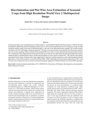
Figure2
Figure 2. Process diagram for APCD process model.
12

– 1.7 nm between the spectral wavelength range: 320 – 1100
nm).
• Handheld GPS (Trimble, Juno SB).
• Survey of India topographical maps (1: 50,000), Police
station maps (1 inch = 1 mile), Cadastral maps (16 inches =
1 mile), District Statistical Handbook, Census data etc.
4. Methodology
The methodology of the work is based on a number of semi
- automated processes such as Generation of Image
Composites, NDCI, ISODATA algorithm, Classification Co-
occurance Statistics and Raster Statistics for Vector. To
achieve the ultimate result the sequential applications of the
above processes have been presented through a process
model (Figure 2) which is termed as Accelerated Plot-based
Crop Discrimination (APCD).
4.1 On screen visual interpretation
Prior to any image classification technique can be applied on
a certain remote sensing imagery, particularly for any kind of
discriminative analysis, it is essential to understand the basic
topographic features of the concerned area .In order to
FCC Crop - A Crop - B Crop - C Crop - D Crop - E Crop - F
Other
cropland
features - I
Other
cropland
features - II
Other
cropland
features - III
Other
cropland
features - IV
AB
Figure3
0
100
200
300
400
500
600
700
800
Costal
Blue
Blue Yellow Green Red Red
Edge
NIR1 NIR2
Digitalnumbervalues
Crop - A
Crop - B
Crop - C
Crop - D
Crop - E
Crop - F
Figure 4
Figure 3. Plot level Visual separation of crops types through composite A and B.
Figure 4. Spectral curve of all crop types generated from WV-2.
Table 1
Normalized Difference Crop Index
Crop (NDCI I) (NDCI II) (NDCI III)
Crop A .037 - .086 .020 - .087 0.10 - 0.28
Crop B .050 - .080 0.10 - 0.14 0.30 - 0.40
Crop C .031 - .088 0.040 - 0.15 0.23 - 0.34
Crop D 0.013 - .023 0.072 - 0.12 0.30 - 0.40
Crop E 0.011 - 0.081 0.11 - 0.19 0.34 - 0.36
Crop F 0.011 - 0.066 0.019 - 0.090 0.12 - 0.25
Table 1. NDCI ranges for different crops.
13

observe the different features present in the WV-2 satellite
data of the study area, ‘False colour composite’ (FCC)
images have been generated along with the true colour image
composite.
Additionally the panchromatic image is also used to observe
the textural pattern of the distinct crop features. Preliminarily
a nomenclature i.e. Crop A, B, C, D, Other cropland features
(OCF I, II, III, IV) etc are assigned to the visually separable
crop and non-crop features based on various tones , textures
and patterns of the composite images(Figure 3).
4.2 Onscreen Spectral separation through
custom band indices
As the visual separation of the crop types is the direct result
of their spectral properties we first generated spectral curve
(Figure 4) for all the visually separable crop features from
the eight bands of WV 2. From that curve we find out the
spectral regions where maximum separation between the
crop features are noticed.
Based on that spectral separation we have computed three
numbers of indices ( NDCI- I, II & III ) using those particular
bands which yielded good normalized differences as well as
enabling us to calculate distinct normalized index ranges
between the crop types (Table 1). These normalized
difference indexes for the purpose of crop discrimination are
termed as ‘Normalized Difference Crop Index’ (NDCI). The
generated three indices are as follows:
NDCI I = (NIR 1 - NIR 2 / NIR1 + NIR 2)
NDCI II = (NIR 1 - Red-Edge / NIR1 + Red-Edge)
NDCI III = (NIR 1 - Green / NIR1 + Green)
These grey scale rasters are minutely compared with
Composites by raster overlay technique to verify the spectral
separation of the crop features by observing and noting the
per pixel values. For each crop feature, 15 to 20 image pixels
are chosen randomly from the associated plots (number of
pixels chosen is directly proportion to the size of the plot).
On an average 4 to 6 plots are chosen for every crop feature.
4.3 Automatic crop-feature extraction by
applying ISODATA algorithm
The ISODATA algorithm is applied subsequent to the visual
and spectral separation for generating the category raster
output utilizing the bands where maximum spectral
separation is achieved. The classification parameters for the
above algorithm are shown bellow –
- Number of classes : 50
- Maximum Iterations : 10
- Maximum Standard Deviation: 4.5000
- Minimum Distance to Combine : 3.2000
- Minimum Cluster Cells : 30
- Minimum Distance for Chaining : 3.2000
The number of classes to be considered is entirely depending
on the variety of features present in the satellite image.
4.3.1 Co-occurrence Statistics and Jeffries-Matusita
distance computation
To observe whether random bias is involved in the
classification process and to judge which classes are spatially
aswellasspectrallyassociatedwitheachother,‘Classification
Co-occurrence Statistics’ (TNTmips tutorial, 2011) is
computed from the category raster output which represents
both the co-occurrence value (upper number) and the
separability value (lower number) for each pair of classes. A
positive co-occurrence value between two classes with a
relatively low separability value indicates that they tend to
occur together in the same spectral space. The normalized
values for above co-occurrence are produced by comparing
the raw frequencies of adjacency with the values expected
from a random distribution of class cells. The ‘Jeffries-
Matusita distance’ based on the ‘Bhattacharya Distance’ is
used to measure the separability of classes, as each pair
represents two probability distributions across the same
spectral space.
4.3.2 Construction of ‘Normalized co-occurrence matrix
A co-occurrence matrix or Gray-Level Co-occurrence
Matrices (GLCM) is a matrix or distribution that is defined
over an image to be the distribution of co-occurring values at
a given offset. Therefore, if ‘I’ be a given grey scale image
and ‘N’ be the total number of grey levels in the image then
the Co-occurrence Matrix is a square matrix ‘G’of order ‘N’,
where the (i, j)th
entry of G represents the number of
occasions, a pixel with intensity, ‘I’ is adjacent to a pixel
with intensity ‘j’, as defined by ‘Haralick’(Alam and Faruqui
2011).
So mathematically, a co-occurrence matrix ‘C’ is defined
over an n × m image ‘I’, parameterized by an offset (Δx,Δy),
as:
Where, i and j are the image intensity values, ‘p’ and ‘q’ are
the spatial positions in the image ‘I’ and the offset (Δx,Δy)
depends on the direction used ‘ᶿ’ and the distance at which
the matrix is computed, ‘d’. As ‘N’ is the total number of
grey levels in the image, thus the normalized co-occurrence
matrix, ‘CN
’ is calculated as:
CN = (1/N) C ∆x ∆y (i, j) ……….. Equation 2
14
occurrence Statistics’ (TNTmips tutorial, 2011) is computed from the category raster output
which represents both the co-occurrence value (upper number) and the separability value
(lower number) for each pair of classes. A positive co-occurrence value between two classes
with a relatively low separability value indicates that they tend to occur together in the same
spectral space. The normalized values for above co-occurrence are produced by comparing
the raw frequencies of adjacency with the values expected from a random distribution of class
cells. The ‘Jeffries-Matusita distance’ based on the ‘Bhattacharya Distance’ is used to
measure the separability of classes, as each pair represents two probability distributions
across the same spectral space.
4.3.2 Construction of ‘Normalized co-occurrence matrix
A co-occurrence matrix or Gray-Level Co-occurrence Matrices (GLCM) is a matrix or
distribution that is defined over an image to be the distribution of co-occurring values at a
given offset. Therefore, if ‘I’ be a given grey scale image and ‘N’ be the total number of grey
levels in the image then the Co-occurrence Matrix is a square matrix ‘G’ of order ‘N’, where
the (i, j)th
entry of G represents the number of occasions, a pixel with intensity, ‘I’ is adjacent
to a pixel with intensity ‘j’, as defined by ‘Haralick’ (Alam and Faruqui 2011).
So mathematically, a co-occurrence matrix ‘C’ is defined over an n × m image ‘I’,
parameterized by an offset (Δx,Δy), as:
∁∆x,∆y(i, j) = ∑ ∑ {
1, if I(p, q) = i and I (p + ∆x, q + ∆y) = j
0, otherwise
m
q=1
n
p=1 .. Equation 1
Where, i and j are the image intensity values, ‘p’ and ‘q’ are the spatial positions in the image
‘I’ and the offset (Δx,Δy) depends on the direction used ‘ᶿ’ and the distance at which the

4.3.3 Bhattacharya distance for measuring separability
of classes
In statistics, the Bhattacharyya distance measures the
similarity of two discrete or continuous probability
distributions or classes by extracting the mean and variances
of two separate distributions or classes.
In its simplest formulation, the Bhattacharyya distance
between two classes under the normal distribution can be
mathematically calculated as:
Where, DB
(p, q) is the Bhattacharyya distance between p
and q distributions or classes,
σp
is the co- variance matrix of the p-th distribution,
σq
is the co- variance matrix of the q-th distribution,
µp
is the mean vector for the p-th distribution
µq
is the mean vector for the q-th distribution and,
p ,q are two different distributions or classes.
4.3.4 Jeffries-Matusita distance for measuring
separability of classes
The Jeffries-Matusita distance (J-M) is a transformation of
the Bhattacharya distance (DB
(p, q)), which has a fixed
range [0, √2]. Here the J-M distance is squared so that the
range lies between 0 and 2. Mathematically the J-M is
calculated as:
Based on the above equations (Eqn.1-4) the ‘Classification
Co-occurrence Statistics’ have been calculated for all the
classes. The classes having high positive co-occurrence (>
50) value with low separability value (< 1.1) are merged
together (Table 2).The final category raster output is reduced
to 12 numbers of classes from the number of 50 classes
(Figure 5).
4.4 Plot based GPS survey and ground truth
verification
A detailed GPS survey followed by farmer’s interview was
carried out during the growing season of the winter crops.
This survey data was compared with the ISODATA output
and accordingly the crop types A, B, C, D were verified as
Mustard, Cauliflower, Brinjal and Cabbage respectively.
Crop classes E and F were identified as Berry and Banana
plantations and that is why their spectral signatures are not
included in the present study. The remaining classes such as
OCFI, II, III and IV were verified as agricultural plots under
preparation for the next crop (Table 3). The information
regarding non crop features such as water body and shadow
areas are not given here.
Table 2
Co-occurrence and Separability analysis
Class Crop A Crop B Crop D Crop C OCFI OCFII OCFIII OCFIV Crop E Crop F
Crop A
188.719,
0.000
Crop B
35.745,
1.116
213.585,
0.000
Crop D
-32.829,
1.880
-19.521,
1.855
231.411,
0.000
Crop C
-52.081,
1.809
-36.919,
1.760
51.491,
1.160
222.719,
2.000
OCFI
-17.000,
1.545
-80.006
1.926
-44.778,
2.000
-69.140,
1.998
257.386,
0.000
OCFII
-55.762,
1.601
-79.767,
1.861
-46.670,
2.000
-72.338,
1.999
-63.831,
1.801
224.811,
0.000
OCFIII
-25.176,
1.324
-69.054,
1.772
-47.389,
1.999
-73.627,
1.986
-21.602,
1.445
-3.093,
1.295
199.706,
0.000
OCFIV
-31.960,
1.853
-41.623,
1.952
-27.463,
2.000
-39.077,
2.000
-38.524,
1.974
33.240,
1.336
-41.202,
1.945
278.692,
0.000
CropE
-10.402,
2.000
-11.988,
2.000
-6.997,
2.000
-9.432,
2.000
-11.493,
2.000
-10.630,
2.000
-12.148,
2.000
13.599,
1.999
266.138,
0.000
CropF
-36.740,
1.929
-36.259,
1.906
12.136,
1.667
11.517,
1.193
-47.979,
1.998
-50.335,
2.000
-51.625,
1.996
-27.496,
1.992
13.090,
1.591
233.385,
0.000
Table 2. Classification Co-occurrence Statistics.
matrix is computed, ‘d’. As ‘N’ is the total number of grey levels in the image, thus the
normalized co-occurrence matrix, ‘CN’ is calculated as:
CN = (1/N) C ∆x ∆y (i, j) ……….. Equation 2
4.3.3 Bhattacharya distance for measuring separability of classes
In statistics, the Bhattacharyya distance measures the similarity of two discrete or continuous
probability distributions or classes by extracting the mean and variances of two separate
distributions or classes.
In its simplest formulation, the Bhattacharyya distance between two classes under the normal
distribution can be mathematically calculated as:
DB(p, q) =
1
4
ln (
1
4
(
σp
2
σq
2
+
σq
2
σp
2
+ 2)) +
1
4
(
(μp
− μp
)2
σp
2 + σq
2
) … . . . . Equation 3
Where, DB(p, q) is the Bhattacharyya distance between p and q distributions or classes,
σp is the co- variance matrix of the p-th distribution,
σq is the co- variance matrix of the q-th distribution,
µ pis the mean vector for the p-th distribution
µ qis the mean vector for the q-th distribution and,
p ,q are two different distributions or classes.
4.3.4 Jeffries-Matusita distance for measuring separability of classes
The Jeffries-Matusita distance (J-M) is a transformation of the Bhattac
q)), which has a fixed range [0, √2]. Here the J-M distance is squared s
between 0 and 2. Mathematically the J-M is calculated as:
J − M = √(1 − e−DB(p,q)) ……….. Equation 4
Based on the above equations (Eqn.1-4) the ‘Classification Co-occu
been calculated for all the classes. The classes having high positive
value with low separability value (< 1.1) are merged together (Tabl
raster output is reduced to 12 numbers of classes from the number of 5
4.4 Plot based GPS survey and ground truth verification
A detailed GPS survey followed by farmer’s interview was carried
season of the winter crops. This survey data was compared with the
accordingly the crop types A, B, C, D were verified as Mustard, C
Cabbage respectively. Crop classes E and F were identified as Berry
and that is why their spectral signatures are not included in the presen
classes such as OCFI, II, III and IV were verified as agricultural plot
the next crop (Table 3). The information regarding non crop features
shadow areas are not given here.15

Figure 5
Figure 5. ISODATA output: category raster with associated classes.
4.5 Accuracy assessment
Error matrix is an effective way to perform classification
error analysis. That is why based on the field information
training cells of known classes were created on the ground
truth raster and compared to their counterparts in the category
raster output. Each row in the error matrix represents a
certain class of the classified output and each column a
ground truth class. The Error matrix (Table 4) shows two
measures of accuracy for individual classes which are User’s
accuracy and Producer’s accuracy. The User’s accuracy
signifies the percentage of cells correctly classified in the
classified output while the Producer’s accuracy shows the
percentage of sample cells correctly classified in the ground
truth raster or training set. The overall accuracy of the
classification process adopted for the APCD model is
calculated as:
100 × (Number of correctly classified raster cells) / (Total
number of cells in ground raster) %
= 100 × (The sum of leading diagonal values) / 10334 (%)
= 100 × (9208 / 10334) (%)
= 89.10 %
The Kappa coefficient is 0.8727. The result indicates a good
deal of efficiency of the classification process.
5. Verification of the WV 2 Image
Discrimination with Hyperspectral Data
5.1 Spectral data acquisition
To cross check the above discrimination a portable field-
spectroradiometer was used to collect spectral signatures of
the same winter crops as it takes measurement of absolute
radiometric quantities in narrow wavelength intervals
irrespective of temporal and spatial variations and provides
valuable assistance in quantifying biophysical characteristics
Table 3
Crop Class number Field information
Crop A 2 Mustard
Crop B 3 Cauliflower
Crop C 4 Cabbage
Crop D 5 Brinjal
Crop E & F 11 & 12 Plantations
Other cropland features 6, 7, 8 & 9 Cropland under preparation
Table 3. Crop types and their associated class information
after field verification.
16

Ground Truth Data
Class Waterbody Mustard Cauliflower Cabbage Brinjal OCFI OCFII OCFIII OCFIV Shadow CropE CropF Total
User’s
accuracy
Waterbody 169 0 0 0 0 0 5 0 0 1 2 15 192 88.02%
Mustard 0
693 42 1 0 3 7 0 1 0 0 0 747 92.77%
Cauliflower 0 28 1049 1 7 0 0 0 0 0 3 4 1092 96.06%
Cabbage 0 0 5 318 290 0 0 0 0 0 21 2 636 50.00%
Brinjal 0 0 1 41 724 0 0 0 0 0 146 46 958 75.57%
OCFI 0 3 0 0 0 1172 17 6 0 0 0 0 1198 97.83%
OCFII 0 0 0 0 0 0 943 6 18 0 0 0 967 97.52%
OCFIII 0 7 0 0 0 15 12 244 0 0 0 0 278 87.77%
OCFIV 0 0 0 0 0 0 23 0 365 0 0 16 404 90.35%
Shadow 16 0 0 0 0 0 0 0 0 32 0 0 48 66.67%
CropE 0 0 0 1 157 0 0 0 0 0 653 66 877 74.46%
CropF 6 0 13 1 18 0 1 0 6 0 46 2846 2937 96.90%
Total 191 731 1110 363 1196 1190 1008 256 390 33 871 2995 10334
Producer’s
accuracy 88.48% 94.80% 94.50% 87.60% 60.54% 98.49% 93.55% 95.31% 93.59% 96.97% 74.97% 95.03%
Table 4
of agricultural crops (Arafat et al.,2013; Blackburn,1998;
Shibayama and. Akiyama,1991; Curran et al.,1990). At least
twenty to twenty-five spectral signatures of each crop were
collected between 11 am to 1 pm at a fixed height of 12 cm
over the leaf (at nadir position, 90 degrees) from the
individual plots along with GPS coordinates. A white
reference Spectralon calibration panel was used at every 20-
25 measurements. Thereafter those spectroradiometer data
were spectrally analyzed and compared with the WV 2 image
data .The curve generated from the spectroradiometer data
(Figure 6) shows similar spectral separability of the crops at
the same spectral region noticed in the image data.
5.2 Co-relation and regression analysis
To statistically verify the above separation regression and
correlation analysis has been done between the three NDCIs
generated from the spectroradiometer data as well as WV-2
imagery which again shows good co-relation in the ‘Linear
Regression Model’ with R2
value for each crop variable
ranges from 0.85 to 0.97 (Table 5).
6. Application of Raster Statistics for Vector
for Plot based crop area calculation
In plot level crop area calculation from high resolution
satellite data the presence of ‘Mixed pixels’ is a major
problem which is generally found along the edges of image
features. In the present ISODATA output the mixed pixels
problem arises due to the spectral conflict between the crops
having relatively similar spectral properties although they
are distinctly different from each other that have been
reflected in the NDCI ranges. Henceforth to solve this
problem and to achieve exact plot wise crop area information
a GIS application named Raster statistics for Vector (RSV)
has been applied on the category raster output using ‘TNT
mips 2014’ software instead of simple attribute transfer,
raster to vector operation or other theoretical approaches
(Czaplewski& Catts,1992). It utilizes the Hough histogram
technique for feature separation and subsequently calculates,
extracts and links the maximum occurring class number
(Mode or majority value) of a particular crop with its
associated polygon from the plot boundary layer. For
example in the present study if a plot gets the mode value ‘2’
from the ISODATA raster through RSV, it means that
particular plot is covered by mustard (Crop A) and its area
will be obtained from the corresponding plot boundary
vector (Figure 7).
7. Results and Discussion
7.1 Visual separation
To understand the visual characteristics of the various crop
features present in the study area from WV 2 a number of
False Colour Composites (FCC) were formed. Out of the
generated composites the two most distinct false colour
composites (Figure 3) where maximum visual separation
between the crop features were observed are:
- Composite –A formed by combining Red-Edge, Green
and Blue and
- Composite – B which was the result of NIR 1, Red-
Table 4. Error matrix of ISODATA classification in APCD process.
Crop
R2
value for
NDCI - I
R2
value for
NDCI - II
R2
value for
NDCI - III
Brinjal 0.911 0.9425 0.949
Mustard 0.928 0.950 0.889
Cauliflower 0.855 0.970 0.937
Cabbage 0.903 0.918 0.910
Table 5
Table 5. Coefficient of determination R2
values for each crop
in the linear regression model.
17

0
10
20
30
40
50
60
70
80
90
Coastal
Blue
Blue Green Yellow Red Red
Edge
NIR1 NIR II
Reflactance
Mustard
Cauliflower
Brinjal
Cabbage
Figure 6 Plot No: 1643
JL No: 80/3
Mode Value: 2
Crop: Mustard
Area Sqr. m: 1265.44
Figure 7
Figure 6. Spectral curve of all crop types generated from Spectroradiometer data.
Figure 7. Final vector output with mode value.
Edge and Green bands respectively.
7.2 Spectral discrimination
Once the visual separation of the crop features is obtained
their spectral nature is known through the generation of
respective spectral curve .The generated spectral curve
(Figure 4) shows that the crop features have greater spectral
discrimination between Red edge, NIR1 and NIR 2 and also
are clearly distinguishable at the Green (VNIR) region of the
spectrum which is very closely matching with visually
separated bands . Accordingly by considering those selected
bands three numbers of indices (NDCI I between NIR 1 -
NIR 2 / NIR1 + NIR 2 , NDCI II between NIR 1 - Red-
Edge / NIR1 + Red-Edge and NDCI III between NIR 1 -
Green / NIR1 + Green) have been generated and from there
18

good normalized differences as well as distinct normalized
index ranges are achieved for the crops (Table 1).
7.3 Statistical analysis of the ISODATA output
The Co-occurrence and Separability analysis (Table 2)
shows that all the visually separable crop features and the
other cropland features are distinctly different from each
other as they have negative to low co-occurrence and high
spectral separabitity between them. The co-occurrence value
is generally greater than 200 and the separability (square of
J-M distance) is expectedly zero (on a scale of 0 – 2) for the
same crop classes. Crops which are visually distinct in the
image composites as well as have different indices ranges
are mostly associated with negative co-occurrence.
Moderately positive spatial and spectral adjacency were
observed between the pair of Mustard and Cauliflower (Co-
occurrence: 35.745, square of J-M distance: 1.116) as well as
for Cabbage and Brinjal (Co-occurrence: 51.491, square of
JM distance: 1.160). Based on the results in Table 2 it can be
predicted that the crops should be discriminable by most of
the pixel based approaches such as ISODATA, Maximum
Likelihood etc. using WV 2.
The ISODATA classification process adopted for the APCD
process model shows an overall accuracy of 89.10% while
the Kappa coefficient is 0.8727.
The Error matrix (Table 4) reveals that the User’s accuracy
and the Producer’s accuracy for all the classes are mostly
above 85% which indicates that each individual class was
correctly classified in both the training raster (ground truth)
and in the ISODATA (classified) output. Among the crops
Mustard and Cauliflower have the highest User’s and
Producer’s accuracy, 92.77%, 94.80% and 96.06%, 94.50%
respectively. Cabbage has the lowest User’s accuracy, 50%,
among the crop classes though its Producer’s accuracy is
significantly higher, 87.60%. For Brinjal the percentage of
cells correctly classified in the ISODATA output is 75.57%
while it’s Producer’s accuracy is lower than that i.e. 60.54%.
Crop E and F which were verified as Berry (in early growth
stage) and Banana plantations respectively have User’s and
Producer’s accuracy of 74.46%, 74.97% and 96.90%,
95.03%.
Table 6
Crop name
Area (Sq.m) obtained
from GPS survey.
Area (Sq.m) obtained
from RSV
Area accurately
estimated (%)
Mustard 22517.95 25508.21 88.28%
Cauliflower 85075.18 91084.23 93.40%
Cabbage 10639.41 12219.97 87.07%
Brinjal 52835.18 57361.52 92.11%
Total Area 172648.28 184593.37 93.53%
Table 6. Crop wise coverage area comparison between RSV and survey data.
Figure 8. Brinjal : image data in X axis and Spectroradiometer
data in Y axis.
Figure9.Mustard:imagedatainXaxisandSpectroradiometer
data in Y axis.
19

The total plot level coverage area of the winter crops i.e.
Mustard, Cauliflower, Brinjal and Cabbage obtained through
RSV (Table 6) is 93.53% of the area calculated from the
detailed plot level GPS survey data. Out of which Cauliflower
and Brinjal has the highest amount of accuracy i.e. 93.40%
and 92.11% respectively.
7.4 Comparison of image data with
Spectroradiometer data
By comparing the spectral curve generated from the image
(Figure 4) as well as spectroradiometer (Figure 6) data we
have noticed that the spectral pattern of all the crops is same
in both the cases with maximum reflection occurring in NIR
1 band . It was also found that indices generated from image
data as well as from spectroradiometer data have good co-
relation in ‘Linear Regression Model’. Out of three NDCIs,
the NDCI-II calculated using NIR I and Red-Edge bands
have greater co-relation with the R² existing between the
values 0.92 to 0.97 (Figure 8 to 11).
8. Conclusion
Figure 10. Cauliflower : image data in X axis and
Spectroradiometer data in Y axis.
Figure 11. Cabbage : image data in X axis and
Spectroradiometer data in Y axis.
The techniques utilized for APCD such as generation of
image composite, NDCI, automatic feature extraction by
ISODATA, classification co-occurrence statistics and RSV,
are all semi-automated processes which require less user
intervention. Not only this through the calculation of
statistical ‘Mode’ over seasonal satellite data one can get an
overview about the agricultural practices carried out in a
certain region which is necessary for agro-economic
development of that particular area. Lastly, based on the
above findings we can conclude that the proposed process is
potentially a time saving and cost effective solution for
generating plot based up-to-date agricultural land use
information database.
Acknowledgement
The authors are thankful to the Principal Secretary,
Department of Science & Technology, Government of West
Bengal for providing funds to carry out the work and to
extend the computational facilities of the Geoinformatics &
Remote Sensing Cell of the Department. The administrative
help of Dr. P.B. Hazra, Senior Scientist, Department of
Science &Technology, Government of West Bengal is also
acknowledged. The authors are thankful to Professor Subash
Santra, Department of Environmental Science, Kalyani
University and Dr. Dipak Ray, Superintendent Engineer,
West Bengal State Electricity Board for providing technical
support.
References
1. Alam, F. I., R. U. Faruqui, (2011). Optimized Calculations
of Haralick Texture Features. European Journal of
Scientific Research, 50 (4); 543-553.
2. Arafat, S. M., M. A. Aboelghar& E. F. Ahmed (2013).
Crop Discrimination Using Field Hyper Spectral
Remotely Sensed Data. Advances in Remote Sensing, 2:
63-70; http://dx.doi.org/10.4236/ars.2013.22009.
3. Banerjee, S., A. Basu., S. Bhattacharya, S. Bose, D.
Chakrabarty& S. S. Mukherjee (2014). Minimum distance
estimation of milky way model parameters and related
inference. http://arxiv.org/pdf/1309.0675.pdf .
4. Beach, R. H., B. J. DeAngelo, S. Rose, C. Li, W. Salas &
S. J. DelGrosso (2008). Mitigation potential and costs for
global agricultural greenhouse gas emissions.Agricultural
Economics, 38: 109-115.
5. Blackburn, G. A., (1998). Spectral indices for estimating
20

photosynthetic pigment concentrations: a test using
enescent tree leaves. International Journal of Remote
Sensing, 19(4):657-675.
6. Curran, P.J., J.L. Dungan & H.L. Gholz (1990). Exploring
the relationship between reflectance red edge and
chlorophyll content in slash pine. Tree Physiology, 7:33--
48.
7. Czaplewski, R.L. and Catts, G.P., 1992. Calibration of
remotely sensed proportion or area estimates for
misclassification error. Remote sensing of Environment,
39, 29 -43.
8. Hayes, M. J. & W. L. Decker (1996). using NOAA
AVHRR data to estimate maize production in the united
states corn belt. International Journal of Remote Sensing,
17(16): 3189-3200; DOI:10.1080/01431169608949138.
9. Image classification with TNTmips, Tutorial, 2011.
Microimages, Inc. http://www.microimages.com/
documentation/Tutorials/classify.pdf
10. Lee, Y. K. & T. R. Bretschneider (2010). Segmentation of
Dual-Frequency Polarimetric SAR Data for an improved
Land Cover Classification. Asian Association on Remote
Sensing, In: 31st Proceedings of Asian Conference on
Remote Sensing (ACRS); http://a-a-r-s.org/acrs/
administrator/components/com_jresearch/files/
publications/ TS13-1.pdf.
11. Leeuw, J. de , Y. Georgiadou, N. Kerle, A. de Gier, Y.
Inoue, J. Ferwerda, M. Smies& D. Narantuya (2010). The
function of remote sensing in support of environmental
policy. Remote Sensing, 2: 1731-1750; DOI:10.3390/
rs2071731.
12. Novotná, K., P. Rajsnerová, P. Míša, M. Míša& K. Klem
(2013). Normalized red-edge index – new reflectance
index for diagnostics of nitrogen status in barley. Mendel
Net, 120-126.
13. Pena- Barragán, J. M., M. K. Ngugi, R. E. Plant & J. Six
(2011). Object-based crop identification using multiple
vegetation indices, textural features and crop phenology.
Remote Sensing of Environment, 115: 1301-1316.
14. Sebastian, B. V., A. Unnikrishnan& K. Balakrishnan
(2012) .Grey level co-occurrence matrices: generalisation
and some new features. International Journal of Computer
Science, Engineering and Information Technology
(IJCSEIT), 2(2): 151-157; DOI: 0.5121/ijcseit.2012.2213.
15. Shibayama, M. & T. Akiyama (1991). Estimating grain
yield by remote sensing of crop of rice canopies using
high spectral resolution reflectance measurements.
Remote Sensing of Environment, 36(1): 45–53.
16. Swain, P. H., T. V. Robertson, & A. G. Wacker (1971).
Comparison of the divergence and b-distance in feature
selection. Information Note: 020871, LARS/Purdue
University, WL, Indiana. http://www.lars.purdue.edu/
home/references/LTR_020871.pdf.
17. Ustunera, M., F. B. Sanli, S. Abdikan, M. T. Esetlili& Y.
Kurucu (2014). Crop type classification using vegetation
indices of RAPIDEYE imagery. The International
Archives of the Photogrammetry, Remote Sensing and
Spatial Information Sciences, XL(7) ISPRS Technical
Commission VII Symposium, Istanbul, Turkey,
DOI:10.5194/isprsarchives-XL-7-195-2014.
18. Wang, C (2008). Detecting invasive sericea lespedeza
(lespedeza cuneata) in missouri pasturelands with hyper-
and multi-spectral aerial photos. American Society for
Photogrammetry and Remote Sensing(ASPRS), Annual
Conference 2008. Portland, Oregon.
19. Wilson, J. H., C. Zhang & J. M. Kovacs (2014).
Separating Crop Species in Northeastern Ontario Using
Hyperspectral Data. Remote Sensing, 6, 925-945; DOI:
10.3390/rs6020925.
21

216-880-1-PB

Recommended

Recommended

More Related Content

What's hot

What's hot (7)

Similar to 216-880-1-PB

Similar to 216-880-1-PB (20)

216-880-1-PB