Delivering nature-based solution outcomes by addressing policy, institutiona...
Remotesensing 11-00164
1. remote sensing
Article
Classification of Land Cover, Forest, and Tree Species
Classes with ZiYuan-3 Multispectral and Stereo Data
Zhuli Xie 1,2, Yaoliang Chen 3,4, Dengsheng Lu 1,2,*, Guiying Li 3,4 and Erxue Chen 5
1 State Key Laboratory of Subtropical Silviculture, Zhejiang A&F University, Hangzhou 311300, China;
xiezhuli_1@163.com
2 School of Environmental & Resource Sciences, Zhejiang A&F University, Hangzhou 311300, China
3 State Key Laboratory for Subtropical Mountain Ecology of the Ministry of Science and Technology and
Fujian Province, Fujian Normal University, Fuzhou 350007, China; chenyl@fjnu.edu.cn (Y.C.);
ligy326@yahoo.com (G.L.)
4 School of Geographical Sciences, Fujian Normal University, Fuzhou 350007, China
5 Institute of Forest Resources Information Technique, Chinese Academy of Forestry, Beijing 100091, China;
chenerx@ifrit.ac.cn
* Correspondence: luds@zafu.edu.cn; Tel./Fax: +86-571-6374-6366
Received: 6 November 2018; Accepted: 12 January 2019; Published: 16 January 2019
Abstract: The global availability of high spatial resolution images makes mapping tree species
distribution possible for better management of forest resources. Previous research mainly focused on
mapping single tree species, but information about the spatial distribution of all kinds of trees,
especially plantations, is often required. This research aims to identify suitable variables and
algorithms for classifying land cover, forest, and tree species. Bi-temporal ZiYuan-3 multispectral and
stereo images were used. Spectral responses and textures from multispectral imagery, canopy height
features from bi-temporal stereo imagery, and slope and elevation from the stereo-derived
digital surface model data were examined through comparative analysis of six classification
algorithms including maximum likelihood classifier (MLC), k-nearest neighbor (kNN), decision tree
(DT), random forest (RF), artificial neural network (ANN), and support vector machine (SVM).
The results showed that use of multiple source data—spectral bands, vegetation indices, textures,
and topographic factors—considerably improved land-cover and forest classification accuracies
compared to spectral bands alone, which the highest overall accuracy of 84.5% for land cover classes
was from the SVM, and, of 89.2% for forest classes, was from the MLC. The combination of leaf-on
and leaf-off seasonal images further improved classification accuracies by 7.8% to 15.0% for land
cover classes and by 6.0% to 11.8% for forest classes compared to single season spectral image.
The combination of multiple source data also improved land cover classification by 3.7% to 15.5%
and forest classification by 1.0% to 12.7% compared to the spectral image alone. MLC provided
better land-cover and forest classification accuracies than machine learning algorithms when spectral
data alone were used. However, some machine learning approaches such as RF and SVM provided
better performance than MLC when multiple data sources were used. Further addition of canopy
height features into multiple source data had no or limited effects in improving land-cover or forest
classification, but improved classification accuracies of some tree species such as birch and Mongolia
scotch pine. Considering tree species classification, Chinese pine, Mongolia scotch pine, red pine,
aspen and elm, and other broadleaf trees as having classification accuracies of over 92%, and larch
and birch have relatively low accuracies of 87.3% and 84.5%. However, these high classification
accuracies are from different data sources and classification algorithms, and no one classification
algorithm provided the best accuracy for all tree species classes. This research implies the same data
source and the classification algorithm cannot provide the best classification results for different
land cover classes. It is necessary to develop a comprehensive classification procedure using an
expert-based approach or hierarchical-based classification approach that can employ specific data
variables and algorithm for each tree species class.
Remote Sens. 2019, 11, 164; doi:10.3390/rs11020164 www.mdpi.com/journal/remotesensing
2. Remote Sens. 2019, 11, 164 2 of 27
Keywords: tree species; classification; ZiYuan-3; stereo image; machine learning
1. Introduction
A substantial decrease of global forest area from unprecedented human disturbance causes
a huge loss of biodiversity [1]. The expansion of plantations compensates this damage to some
extent. Plantations provide some habitat needs for a subset of animal species and diverse timbers
for human use. Understanding the distribution of plantations is very important in biodiversity
assessment [2], forest biomass prediction [3,4], ecosystem services and biogeochemical cycling [5–7],
and forest resources management [8]. China, as the largest plantation area in the world since 1999 [9],
experienced a dramatic increase from nearly 47 million hectares in 1999 to nearly 70 million hectares in
2014 [10], which requires timely updates of spatial information of forest distribution. Depending on
the geolocations and climate zones in China, the spatial patterns, and types of plantations vary such as
rubbers in a tropical region of south China, eucalyptus in a subtropical region in east and south China,
Chinese fir plantations in the subtropical region, and different kinds of pines (e.g., larch, Chinese pine,
red pine) in north China. Plantations have played more and more important roles in improving
economic conditions for local persons.
Remotely sensed data has long been used for land-cover mapping in large areas due to the
unique characteristics of spectral, temporal, and spatial features and a digital number data format
suitable for computer processing. Satellite data, such as Landsat, have been explored extensively
for land cover mapping, and even individual tree species mapping, because the data are freely
available and contain a broad range of suitable spectral bands [11–14]. Dong et al. [15] combined
multi-temporal Landsat images and PALSAR (Phased Array type L-band Synthetic Aperture Radar)
data to map rubber tree distribution in China’s Hainan Province and achieved an overall accuracy of
92%. Qiao et al. [16] applied time-series normalized difference vegetation index (NDVI) images from
annual Landsat images over 15 years to identify eucalyptus in Guangdong Province and obtained
an accuracy of 91%. In previous research, single-date images were mostly used because of the
difficulty in obtaining images of different seasons due to poor weather conditions, especially in
tropical and subtropical regions [17,18]. Seasonal vegetation information has proven valuable in
improving vegetation classification [19]. In the subtropical Lin’an District mountains, Xi et al. [20]
used multi-temporal Landsat images to extract hickory plantations by developing subpixel indices
from linear spectral mixture analysis. Because of its relatively coarse spatial resolution in Landsat,
accurate mapping of plantation distribution due to a small parch size become a challenge.
In recent years, attention has shifted to using high spatial resolution satellite data for
detailed classification because of its better ability to capture fine characteristics of objects [21–23].
Gomez et al. [17] used QuickBird multispectral and panchromatic images to extract coffee plantations
in NewCaledonia and obtained an accuracy of 96.9%. Cho et al. [24] applied WorldView-2 images to
extract three tree species in South Africa and obtained an accuracy of 89.3%. Wang and Lu [25] used
the expert-rule based approach based on Chinese Gaofen (GF-1) and ZiYuan (ZY-3) satellite images to
successfully map Torrya forest distribution with an overall accuracy of 84.4%. High spatial resolution
data with multi-temporal features are especially valuable for improving vegetation classification
accuracy [19]. Reis and Tasdemir [26] applied QuickBird data during the growing and deciduous
seasons to identify hazelnut in northeastern Turkey and found that accuracy increased by 9% compared
to using single-season data. Li et al. [19] used four-seasonal GF-1 images to map wetland classification
in Hangzhou Way, China using the expert-based approach with an overall classification accuracy of
90.3%. However, processing and analysis of high spatial resolution satellite data also pose challenges
in terms of large file sizes, canopy shadows, and high spectral variation within the forested areas.
The selection of suitable variables from remotely sensed data is one of the critical steps in
improving classification accuracy [27]. Since high spatial resolution data often have limited spectral
3. Remote Sens. 2019, 11, 164 3 of 27
information. The incorporation of spatial-based variables into spectral features becomes critical [19,21].
Pixel-based features can be individual spectral bands, vegetation indices, or transformed images.
Spatial-based features can be textural images or segmentation [27]. Many previous studies indicated
that combinations of spectral and spatial features improved classification accuracy [18,28] and the
object-based classifier provided better accuracy than pixel-based approaches when high spatial
resolution images were used [21,23,29,30]. Dihkan et al. [31] found that overall accuracy was
improved from 93.82% to 97.40% after integration of textures and multispectral images for mapping
tea plantations using a support vector machine (SVM).
For forest classification, use of the forest stand structure features may support the separation of
different tree species or forest types due to the difference in tree species composition, crown size and
shape, and tree density [32,33]. One critical step is to extract suitable forest attributes such as canopy
height and crown size. The height information was found to be useful in improving classification
accuracy of tree species [34–37]. Holmgren et al. [34] compared the results of mapping tree species in
southern Sweden by separately using three variable conditions (only height information from lidar,
only variables from multispectral data, and a combination of height information and variables from
multispectral data) and found that spectral variables combined with height information provided
the highest accuracy. Ke et al. [36] also found that adding height information improved tree species
mapping accuracy by 3%. In reality, use of height information in forest classification is still very limited
in previous research due to the difficulty in obtaining height images in a large area, but could be an
important factor in improving forest classification in the future because of the availability of lidar and
satellite stereo images.
Many classifiers from statistical-based algorithms—e.g., cluster analysis [38], maximum
likelihood classifier (MLC) [26]—to machine learning algorithms—e.g., decision tree (DT) [36],
artificial neural networks (ANN) [17], SVM [39], expert rules-based approach [25], and random
forest (RF) [37,40]—have been used for land-cover classification based on high spatial resolution
imagery. Previous research implies that the choice of the best classifiers depends mainly on the specific
study area, data, and land-cover classification system [19,27]. Raczko and Zagajewski [41] compared
three machine learning classifiers in identifying five tree species and found that ANN achieved the
highest accuracy. Li et al. [19] applied MLC, RF, and the expert rules-based approach to classify nine
land-cover classes from four seasons of GF-1 multispectral images in Hangzhou Bay coastal wetland.
An accuracy of 90.3% was obtained using the expert rules-based approach. Recent research explored
the use of deep learning in tree species mapping [42–44]. However, more investigation is needed for
this method since it is highly complex and is computationally intensive.
Forest inventories at the county or forest farm scale in China in the 1980s and 1990s were usually
conducted at 10-year intervals using field surveys, topographic maps, and aerial photographs to
create detailed forest distribution maps of tree species, especially for plantations, and to make
plans for forest management. Entering the 2000s, as high spatial resolution satellite images such
as QuickBird, SPOT, and WorldView became widely available, forest inventory was mainly based on
visual interpretation of the images with support from field surveys. Because these processes were time
consuming and labor intensive, and updating and incorporating data from previous inventories was
difficult, research in recent years has shifted to computer-based automatic classification based on the
satellite images. Although the important role of using high spatial resolution images in improving
the quality of mapping forest distribution has been recognized, they have not been extensively used
in real applications. Three major reasons may account for this: (1) the difficulty of using automatic
classification of forest types within existing classification approaches, (2) the limitation of spectral
wavelengths (usually only visible and NIR bands) resulting in the challenge of separation of tree
species, and (3) the costs of image purchase, purchase of computers that can deal with large volumes
of data, and hiring data-processing professionals. However, high spatial resolution data will play an
increasingly important role in the future, for producing detailed forest classification and conducting
forest inventory at local and regional scales.
4. Remote Sens. 2019, 11, 164 4 of 27
Although many studies explored tree species classification using high spatial resolution images,
they mainly focused on single tree species without taking multiple tree species into account.
Many variables from spectral signatures, vegetation indices, texture, and ancillary data can be used
for tree species classification. However, not all variables are needed and improper combinations
of different variables may yield poor classification results. Overfitting in the machine learning
algorithms is also a problem. To date, it is still unclear which classification algorithm provides
the best performance and how different seasonal features, and different data sources influence land
cover or forest classification. The objectives of this research are to explore (1) the incorporation of
different seasonal data (leaf-on, leaf-off), (2) combination of different kinds of variables (spectral,
vegetation indices, textures, shape variables, topographic factors, and height features), and (3)
different classifiers (MLC, ANN, k-nearest neighbor (kNN), DT, RF, and SVM) in improving land
cover (all forest and non-forest classes), forest (all tree species classes), and tree species mapping
performance. Therefore, high spatial resolution multi-spectral and panchromatic data, satellite stereo
images, and topographic data were selected in a plantation-dominated study area in north China.
The contribution of this research is to identify the best classification procedures for land cover, forest,
and tree species classification using high spatial resolution images through comparative analysis of
the classification results based on different scenarios. Other contributions include the calculation
of textural images based on segmented polygons instead of traditional approaches based on fixed
window sizes and the use of canopy height features in improving forest and tree species classification
accuracies. This research will provide new insights on how to select suitable variables and classification
algorithms for land cover and forest classification, especially in temperate monsoon climate regions.
2. Materials and Methods
2.1. Study Area
In order to explore the classification performance using different data sources and classification
algorithms, selection of a typical study area is important. Wangyedian Forest Farm with a total area of
approximately 500 km2, which is located in southwestern Kelaqin, Inner Mongolia, China, was an ideal
study area because of its spatial distribution of typical coniferous forest plantations in a temperate
climate zone (Figure 1). Plantation types mainly include four needle forests (larch, Chinese pine,
Mongolia scotch pine, and red pine) and three deciduous broadleaf forests (birch, aspen, and elm) [45].
Aspen and elm are mainly distributed along roads and around villages, while birch is in the
mountainous areas. This study area is located at relatively high elevations of 1810 m in the west and
783 m in the east (Figure 1). The region has a typical middle continental temperate monsoon climate
with four seasons: dry with frequent wind in the spring, wet and hot in the summer, frequent frosts in
the fall, and cold with a little snow in the winter [46]. Average annual temperatures range from 3.5 ◦C
to 7 ◦C and average annual rainfall is around 400 mm [47].
Founded in 1956 and managed by the former State Forestry Administration until 1978, this farm
was administratively incorporated to Chifeng City. Because it is a state property, management has
focused on afforestation, and harvesting has been strictly prohibited. In 1956, this forest farm had
natural forest areas of about 7300 ha [48]. Between 1956 and 1990, about 15,300 ha of man-made forests
were planted, and, between 1991 and 2006, the emphasis was on the intensive forest management for
the young and middle-age plantations in order to improve the forest quality. After 2007, harvesting of
natural forests was prohibited. By 2014, the forested area was over 22,000 ha, with plantations
accounting for almost half of it [49].
5. Remote Sens. 2019, 11, 164 5 of 27
Remote Sens. 2018, 10, x FOR PEER REVIEW 5 of 29
Figure 1. Study area: Wangyedian Forest Farm in eastern Inner Mongolia, China.
2.2. Data Preparation
2.2.1. Field Survey Data Collection
Datasets used in this study include field survey data and ZiYuan (ZY-3) multispectral,
panchromatic, and stereo data (Table 1). We first designed the sites for the field survey based on the
high spatial resolution image and previous forest map in this study area. During the field work, we
recorded all land cover types around each site. We then digitized all recorded land cover types on
the google earth image and formed a shape file format file. The land covers recorded include larch,
Chinese pine (CP), Mongolia scotch pine (MSP), red pine (RP), birch, aspen, elm, other broadleaf tree
species (OBL), shrub, grass, farmland (FL), bare land (BL), impervious surface area (ISA), and water.
Based on our research objectives and consideration of the separability of land-cover types, a
classification system with 13 land-cover types including seven tree species (larch, CP, MSP, RP, birch,
aspen, and elm (AAE), OBL) designated as forest, and shrub, grass, FL, BL, ISA, and water—were
defined. According to this classification system, the classification results were analyzed on three
levels—land cover (all 13 classes), forest (all seven tree species classes), and tree species (each tree
species class).
Table 1. Data used in the research.
Data Data Description Data Acquisition Dates
Field survey
data
A total of 112 sites were investigated, for which all land covers around
each site were recorded, digitized, and saved in a shape file format.
Thus, over 1000 samples covering different land covers were collected.
September 2017
ZiYuan-3
satellite
data
Four multispectral bands (blue, green, red, and near infrared (NIR)): 5.8
m spatial resolution;
One panchromatic band: 2 m spatial resolution;
9 February 2015: sun elevation
angle of 31.44° and azimuth
angle of 163.06°;
Figure 1. Study area: Wangyedian Forest Farm in eastern Inner Mongolia, China.
2.2. Data Preparation
2.2.1. Field Survey Data Collection
Datasets used in this study include field survey data and ZiYuan (ZY-3) multispectral,
panchromatic, and stereo data (Table 1). We first designed the sites for the field survey based on the high
spatial resolution image and previous forest map in this study area. During the field work, we recorded
all land cover types around each site. We then digitized all recorded land cover types on the google
earth image and formed a shape file format file. The land covers recorded include larch, Chinese pine
(CP), Mongolia scotch pine (MSP), red pine (RP), birch, aspen, elm, other broadleaf tree species (OBL),
shrub, grass, farmland (FL), bare land (BL), impervious surface area (ISA), and water. Based on our
research objectives and consideration of the separability of land-cover types, a classification system
with 13 land-cover types including seven tree species (larch, CP, MSP, RP, birch, aspen, and elm (AAE),
OBL) designated as forest, and shrub, grass, FL, BL, ISA, and water—were defined. According to this
classification system, the classification results were analyzed on three levels—land cover (all 13 classes),
forest (all seven tree species classes), and tree species (each tree species class).
Table 1. Data used in the research.
Data Data Description Data Acquisition Dates
Field survey data
A total of 112 sites were investigated, for which all land covers around
each site were recorded, digitized, and saved in a shape file format.
Thus, over 1000 samples covering different land covers were collected.
September 2017
ZiYuan-3 satellite data
Four multispectral bands (blue, green, red, and near infrared (NIR)):
5.8 m spatial resolution;
One panchromatic band: 2 m spatial resolution;
Stereo images: nadir-view image with 2 m, backward and forward
views with 3.5 m spatial resolution
9 February 2015: sun elevation angle of 31.44◦ and
azimuth angle of 163.06◦;
20 September 2017: sun elevation angle of 44.22◦ and
azimuth angle of 148.18◦
2.2.2. ZiYuan-3 Satellite Data Collection and Pre-Processing
Because of the good data quality, high spatial resolution, and the availability of multi-spectral
and stereo data (Table 1), ZY-3 satellite data are increasingly used in land-cover classification [50–52].
Ideally, different seasonal images in a year will be valuable for mapping forest distribution. After we
6. Remote Sens. 2019, 11, 164 6 of 27
searched all images within three years, we find only two cloud-free images that were acquired in
leaf-on and leaf-off season each, but they were not from the same year. Therefore, two scenes of ZY-3
images, which were acquired on 27 September, 2017 (leaf-on season) and on 9 February, 2015 (leaf-off
season) were used. Figure 2 shows different representations of four kinds of tree species classes on
leaf-on and leaf-off ZY-3 color composites. The ZY-3 stereo images from the same dates were used to
produce digital surface model (DSM) data for this study area. In order to convert digital number data to
surface reflectance in the ZY-3 multispectral images, the dark-object subtraction approach [53] was used
for atmospheric calibration. Because previous research showed that the C-correction model [54,55]
is suitable for images with steep slope terrains and low sun zenith angle [56], we used this method
for topographic correction. In order to make full use of different features in multi-spectral and
panchromatic data, it is necessary to identify suitable data fusion algorithms to conduct this data
fusion. The Gram-Schmidt tool is regarded as a good fusion technique that can improve spatial
information while minimizing spectral distortion [57,58]. Thus, this method was used to integrate
multi-spectral and panchromatic data to produce a new dataset with a spatial resolution of 2 m.
Remote Sens. 2018, 10, x FOR PEER REVIEW 6 of 29
Stereo images: nadir-view image with 2 m, backward and forward
views with 3.5 m spatial resolution
20 September 2017: sun
elevation angle of 44.22° and
azimuth angle of 148.18°
2.2.2. ZiYuan-3 Satellite Data Collection and Pre-Processing
Because of the good data quality, high spatial resolution, and the availability of multi-spectral
and stereo data (Table 1), ZY-3 satellite data are increasingly used in land-cover classification [50–52].
Ideally, different seasonal images in a year will be valuable for mapping forest distribution. After we
searched all images within three years, we find only two cloud-free images that were acquired in leaf-
on and leaf-off season each, but they were not from the same year. Therefore, two scenes of ZY-3
images, which were acquired on 27 September, 2017 (leaf-on season) and on 9 February, 2015 (leaf-
off season) were used. Figure 2 shows different representations of four kinds of tree species classes
on leaf-on and leaf-off ZY-3 color composites. The ZY-3 stereo images from the same dates were used
to produce digital surface model (DSM) data for this study area. In order to convert digital number
data to surface reflectance in the ZY-3 multispectral images, the dark-object subtraction approach [53]
was used for atmospheric calibration. Because previous research showed that the C-correction model
[54,55] is suitable for images with steep slope terrains and low sun zenith angle [56], we used this
method for topographic correction. In order to make full use of different features in multi-spectral
and panchromatic data, it is necessary to identify suitable data fusion algorithms to conduct this data
fusion. The Gram-Schmidt tool is regarded as a good fusion technique that can improve spatial
information while minimizing spectral distortion [57,58]. Thus, this method was used to integrate
multi-spectral and panchromatic data to produce a new dataset with a spatial resolution of 2 m.
Figure 2. A comparison of color composites in leaf-on season (1) and leaf-off season (2) showing
different representations of four tree species classes: birch (a) Chinese pine (b) a composite of different
broadleaf tree species (c) and larch (d).
Figure 2. A comparison of color composites in leaf-on season (1) and leaf-off season (2) showing
different representations of four tree species classes: birch (a) Chinese pine (b) a composite of different
broadleaf tree species (c) and larch (d).
2.2.3. Development of Digital Surface Model Data from Stereo Images
The digital elevation model (DEM) data with high spatial resolution are needed for topographic
correction in this research. However, this kind of data is not available. Thus, we developed
DSM data from ZY-3 stereo images using the Geomatica PCI software with the following steps:
(1) Relative orientation was conducted to create a surface three-dimensional model. The rational
polynomial coefficients (RPC) parameter file was used to locate the relative position between two
different views [59]. (2) Absolute orientation was then conducted to fix the geometric location of
a three-dimensional model in the ground measurement coordinate system by translating, rotating,
and scaling based on selected ground control points (GCPs) [60,61]. (3) Tie points connecting two
images were created to establish a relationship between them. An initial DSM was subsequently
established as well as the errors of tie points and GCPs. If the error was too large, we eliminated
tie points with large errors and recalculated the model. (4) An epi-polar image was developed and
7. Remote Sens. 2019, 11, 164 7 of 27
its corresponding DSM was extracted [62]. Two combinations of views—nadir and backward views,
nadir and forward views—were used to extract the DSM. In order to test the accuracy of the extracted
DSM, 65 points with flat topography (e.g., at a crossroad and in the farmland area) were selected from
Google Earth maps. Results showed that the mean errors in the DSM at leaf-on and leaf-off seasons
were 4.47 and 3.75 m, respectively. The DSM data at the leaf-on season were used for topographic
correction. The DSM data from the leaf-off season were not used for topographic correction due to the
different impacts of deciduous and evergreen forests on DSM data.
Previous research used both DSM images from the leaf-on and leaf-off seasons to produce
a canopy height image [59]. However, for this research, we called this kind of differencing image as
relative canopy height (RCH), considering the different effects of deciduous and evergreen forests.
For deciduous forests, the difference of both DSMs from leaf-on and leaf-off seasons can be assumed
as the canopy height. However, for the evergreen forests, the differencing image cannot represent
the canopy height. Figure 3 shows the developed DSM images from leaf-on and leaf-off seasons,
as well as the RCH image (Figure 3C) from the difference of both DSM images. As a comparison,
we also included a color composite (Figure 3D) using the ZY-3 multi-spectral image at leaf-on season
at the same site and added some specific forest types (e.g., a: birch, b: Mongolia scotch pine, c:
other broadleaf, d: Chinese pine, and e: larch) to show the impacts of deciduous and evergreen forest
types on the RCH values. Although the RCH image cannot represent the real canopy height values of
different forest types, Figure 3 indicates that proper use of this feature may be helpful for improving
forest classification or forest and non-forest separation.
Remote Sens. 2018, 10, x FOR PEER REVIEW 8 of 29
Figure 3. A comparison of the digital surface model (DSM) images from leaf-on season (A) and leaf-
off season (B). The difference between DSMs was used to produce a relative canopy height (RCH)
image, especially for a deciduous forest (C). As a comparison with the RCH image, a color composite
(D) using the ZiYuan-3 multispectral image at the leaf-on season at the same site was provided (a:
birch, b: Mongolia scotch pine, c: other broadleaf, d: Chinese pine, and e: larch). The blue color in
locations ①, ②, ③, and ④ indicates deforestation sites of plantations between 2015 and 2017.
2.2.4. Development of the Segment Image
Previous research shows that the object-based classification approach provided better land cover
accuracy than pixel-based approaches when high spatial resolution images were used [19,21,23].
Pixel-based approaches classify each pixel into only one class based on the digital value of each pixel,
and are very commonly used, especially when medium spatial resolution images such as Landsat
were used [27,63,64]. However, pixel-based approach may produce poor classification results when
very high spatial resolution images are used because of high spectral variation within the same land
cover type [21,22]. In the object-based approach, one critical step is to develop a suitable segment
image. In our research, we used the eCognition software, in which four key parameters—weight of
input layers, weight of spectra and shape, weight of compacts and smoothness, and scale of
segment—need to be carefully defined in the segmentation procedure. Generally, the sum of spectra,
Figure 3. A comparison of the digital surface model (DSM) images from leaf-on season (A) and
leaf-off season (B). The difference between DSMs was used to produce a relative canopy height (RCH)
image, especially for a deciduous forest (C). As a comparison with the RCH image, a color composite
(D) using the ZiYuan-3 multispectral image at the leaf-on season at the same site was provided (a:
birch, b: Mongolia scotch pine, c: other broadleaf, d: Chinese pine, and e: larch). The blue color in
locations 1
, 2
, 3
, and 4
indicates deforestation sites of plantations between 2015 and 2017.
8. Remote Sens. 2019, 11, 164 8 of 27
2.2.4. Development of the Segment Image
Previous research shows that the object-based classification approach provided better land cover
accuracy than pixel-based approaches when high spatial resolution images were used [19,21,23].
Pixel-based approaches classify each pixel into only one class based on the digital value of each pixel,
and are very commonly used, especially when medium spatial resolution images such as Landsat were
used [27,63,64]. However, pixel-based approach may produce poor classification results when very
high spatial resolution images are used because of high spectral variation within the same land cover
type [21,22]. In the object-based approach, one critical step is to develop a suitable segment image.
In our research, we used the eCognition software, in which four key parameters—weight of input
layers, weight of spectra and shape, weight of compacts and smoothness, and scale of segment—need
to be carefully defined in the segmentation procedure. Generally, the sum of spectra, shape weights,
sum of compact, and smoothness should be 1. In this study, shape weight and compact weight were
set as 0.2 and 0.5, respectively, after a substantial number of adjustments. The scale of the segment also
needs to be optimized by continuously checking the segment result and setting it as 100. According to
the optimization, if the scale is too large, aspen, elm, and grass cannot be separated well. In contrast,
if the scale is too small, the segmented polygons will be too fragmented. Based on the developed
segment image, all variables such as vegetation indices and textures were extracted, according to this
segment image.
2.2.5. Framework of This Research
The framework of the mapping land cover, forest, and tree species distribution using ZY-3 data is
illustrated in Figure 4. This framework includes five major steps: (1) data collection and preprocessing,
(2) extraction and identification of variables from ZY-3 data, (3) selection of suitable classifiers,
(4) design of classification scenarios and implementation of image classification corresponding to each
scenario, and (5) validation of classification results.
Remote Sens. 2018, 10, x FOR PEER REVIEW 9 of 29
shape weights, sum of compact, and smoothness should be 1. In this study, shape weight and
compact weight were set as 0.2 and 0.5, respectively, after a substantial number of adjustments. The
scale of the segment also needs to be optimized by continuously checking the segment result and
setting it as 100. According to the optimization, if the scale is too large, aspen, elm, and grass cannot
be separated well. In contrast, if the scale is too small, the segmented polygons will be too fragmented.
Based on the developed segment image, all variables such as vegetation indices and textures were
extracted, according to this segment image.
2.2.5. Framework of This Research
The framework of the mapping land cover, forest, and tree species distribution using ZY-3 data
is illustrated in Figure 4. This framework includes five major steps: (1) data collection and
preprocessing, (2) extraction and identification of variables from ZY-3 data, (3) selection of suitable
classifiers, (4) design of classification scenarios and implementation of image classification
corresponding to each scenario, and (5) validation of classification results.
Figure 4. Framework of mapping land cover, forest, and tree species distribution through a
comparative analysis of classification results using different classification algorithms based on
various scenarios from ZiYuan-3 (ZY-3) data.
Figure 4. Framework of mapping land cover, forest, and tree species distribution through a comparative
analysis of classification results using different classification algorithms based on various scenarios
from ZiYuan-3 (ZY-3) data.
9. Remote Sens. 2019, 11, 164 9 of 27
2.3. Extraction of Potential Variables and Selection of Optimal Variable Combination
In remote sensing optical sensor data, the spectral, spatial, temporal, and subpixel features
are extensively used for land-cover classification [26]. In this research, five kinds of features were
considered: (1) pixel-based spectral features such as spectral signatures and vegetation indices,
(2) spatial-based features such as textural images and image segmentation, (3) temporal features
such as growing and deciduous seasons, (4) height-based variables that can reflect the difference of
forest stand structures, and (5) topographic factors such as slope and elevation.
2.3.1. Extraction of Spectral-Based Variables
Spectral data—spectral bands, vegetation indices, and transformed images—are commonly
used for land-cover classification [27]. In this research, spectral data include four original bands
(blue, green, red, and NIR), the sum of four bands, ratio of each band to the sum of four bands, and
different vegetation indices, which are summarized in Table 2. In order to use temporal information,
differences between specific bands of bi-temporal images and differences between vegetation indices
(VDVI(diff) and NDGI(diff), respectively) were also used.
Table 2. Vegetation indices used in this research.
Vegetation Indices Equations References
Differenced vegetation index (DVI) NIR − Red [65]
Infrared percentage vegetation index (IPVI) NIR/(NIR + Red) [66]
Normalized difference vegetation index (NDVI) (NIR − Red)/(NIR + Red) [65]
Normalized difference greenness index (NDGI) (Green − Red)/(Green + Red) [65]
Normalized difference water index (NDWI) (Green − NIR)/(Green + NIR) [65]
Ratio vegetation index (RVI) NIR/Red [25]
Re-normalized difference vegetation index (RDVI) (NIR − Red)/
p
(NIR + Red) [4]
Visible-band difference vegetation index (VDVI)
((Green − Red)+(Green − Blue))
(Green +Red+Green+ Blue)
[67,68]
Optimized soil adjusted vegetation index (OSAVI) (NIR − Red)/(NIR + Red + 0.16) [4]
Ratio of near-infrared (NIR) band to blue band NIR/Blue [25]
2.3.2. Extraction of Spatial-Based Variables
Spatial features are important for high spatial resolution images and are used for
land-cover classification [23,27]. Common spatial features are textures and segmentation.
Traditionally, textures are calculated with a fixed window size (e.g., 3 × 3, 5 × 5) based on a spectral
band. However, because of the difference in patch sizes among land-cover types and locations,
it is difficult to identify optimal textural images that are suitable for different land covers [28].
In order to avoid this problem that no one optimal window size is available for different patch
sizes of land covers, we calculated textural images based on the segmented objects using the
gray-level co-occurrence matrix (GLCM) measures. Eight texture measures (mean, standard deviation,
homogeneity, contrast, dissimilarity, entropy, second moment, and correlation) [69] were calculated in
this research. Another important spatial feature is based on the segmented polygons, including length,
width, area, ellipse, rectangle, shape index, brightness, and border index that they are directly provided
from the segmented results using eCognition software [70,71].
2.3.3. Extraction of Forest Stand Based Variables
Different tree species have their own crown sizes, canopy density, and vertical structure.
Effective use of forest stand structure features is regarded as an important approach to improve
tree species or forest type separation [33]. In this research, an RCH image was extracted from the
difference of DSM data between leaf-on and leaf-off seasons based on the assumption that leaf-on DSM
represents canopy height and leaf-off DSM represents ground elevation [59]. From the RCH image
(see Figure 3(3)), the variables reflecting the difference of forest stand features were then extracted
using the GLCM measures based on the segmented polygons.
10. Remote Sens. 2019, 11, 164 10 of 27
2.3.4. Extraction of Topographical-Based Variables
Topography is related to tree species distribution and topographic factors such as elevation, slope,
and aspect, which are often used to support forest classification [27]. This research selected leaf-on
DSM data from ZY-3 stereo images for calculation of slope, aspect, and elevation. These factors were
used as extra variables by combining them with remote sensing variables for land-cover classification.
2.3.5. Selection of Suitable Variables Using Random Forest
Although many variables can be extracted, they are not all needed for land-cover or forest
classification. The best combination of variables must be identified. Thus, the RF approach was used
because it can provide rankings of variable importance [4]. The selection of variables using the RF
approach was conducted using R software. For each decision tree of RF, the out-of-bag (OOB) error was
calculated (errOOB1) and random noise was added into a certain variable X of OOB from all samples
(errOOB2). The importance of variable X is assumed as the mean value of the sum of differences
between errOOB2 and errOOB1 in all trees. If variable X has a great influence on the classification
result, the OOB accuracy will be considerably reduced after adding random noise, which indicates its
high importance [70]. Pearson’s correlation analysis of the selected variables using RF was conducted
after the importance ranking. For two variables having a correlation coefficient of greater than 0.8,
the one having lower importance ranking was removed if removal of this variable did not produce
a higher error in the RF procedure. All variables were checked during this process, and the selected
variables were not highly correlated to one another.
Table 3 summarized the selected variables using RF based on different data scenarios—leaf-off,
leaf-on, and the combination of those seasons. V1off, V1on, and V1both represent the spectral
bands only at leaf-off, leaf-on, and combination of both seasons. The selected variables in V2off,
V2on, and V2both included spectral responses (spectral band or vegetation index), textural images,
and topographic factors, which implies the importance of using multiple source data in land-cover
classification. Considering scenario V3, three and two forest stand variables corresponding to V3off
and V3on and one forest stand variable corresponding to V3both were selected, which implies that
forest stand structure may be useful in improving land-cover, especially tree species classification.
Table 3. Selected variables for use in land-cover classification.
Data Variables
Data from leaf-off season
V1off BlueF, GreenF, RedF, NIRF.
V2off
NDVIF, Brightness, NDGIF, Slope, NIRF, Elevation, TF-Cor-NIR,
TF-Cor-Green, VDVIF, Aspect, TF-Hom-Red, TF-Hom-Blue, TF-Std-Red.
V3off
NDVIF, RCH, Brightness, NDGIF, Slope, NIRF, Elevation, TF-Cor-NIR,
TF-Cor-Green, VDVIF, TEnt-RCH, Aspect, TF-Hom-Red, TDis-RCH,
TF-Hom-Blue, TF-Std-Red.
Data from leaf-on season
V1on BlueS, GreenS, RedS, NIRS.
V2on
SUMS-all-band, VDVIS, TS-Sec-Blue, NIR/SUMS-all-band, NIR/BLUES,
NIRS, Elevation, TS-Std-Red, TS-Hom-NIR, NDGIS, Slope, TS-Dis-NIR,
TS-Con-Red, TS-Ent-NIR, Length/Width.
V3on
SUMS-all-band, VDVIS, TS-Sec-Blue, NIR/SUMS-all-band, NIR/BLUES,
NIRS, Elevation, TS-Std-Red, TS-Hom-NIR, RCH, NDGIS, Slope, TS-Dis-NIR,
TS-Con-Red, TSec-RCH, TS-Ent-NIR, Length/Width.
Combined data from both seasons
V1both BlueF, GreenF, RedF, NIRF, BlueS, GreenS, RedS, NIRS.
V2both
IPVIF, SUMS-all-band, IPVIS, VDVIS, NIRS, TS-Sec-Blue, NDGI (diff),
NDGIS, TS-Hom-NIR, VDVI (diff), Slope, TS-Ent-Blue, VDVIF, Elevation,
TS-Cor-Red, NDGIF, TS-Std-NIR.
V3both
IPVIF, SUMS-all-band, IPVIS, VDVIS, NIRS, TS-Sec-Blue, NDGI (diff),
NDGIS, RCH, TS-Hom-NIR, VDVI (diff), Slope, TS-Ent-Blue, VDVIF,
Elevation, TS-Cor-Red, NDGIF, TS-Std-NIR.
Note: F, ZiYuan-3 multispectral data in February, NIR, near infrared, NDVI, normalized difference vegetation
index, NDGI, normalized difference greenness index, T, texture, VDVI, visible-band difference vegetation index,
RCH, relative canopy height, S, ZiYuan-3 multispectral data in September, IPVI, infrared percentage vegetation
index, different texture measures: Cor, correlation, Ent, entropy, Hom, homogeneity, Dis, dissimilarity, Std, standard
deviation, Sec, second moment, Con, contrast, different vegetation indices: NDVI = (NIR-Red)/(NIR + Red),
NDGI = (Green-Red)/(Green + Red), VDVI = ((Green-Red) + (Green-Blue))/(Green + Red + Green + Blue),
IPVI = NIR/(NIR + Red), NDGI(diff) = NDGIS-NDGIF, VDVI(diff) = VDVIS-VDVIF.
11. Remote Sens. 2019, 11, 164 11 of 27
2.4. Comparative Analysis of Classification Algorithms
2.4.1. A Brief Description of Six Classification Approaches
Although many classification approaches are available, the one that can provide the best
classification result for a specific study area is unclear. In reality, several classifiers are often selected
for a comparative analysis of the results [63,64]. In this research, six classifiers—maximum likelihood
classifier (MLC), k-nearest neighbor (kNN), decision tree (DT), random forest (RF), artificial neural
network (ANN), and support vector machine (SVM)—were selected. Three classifiers—MLC, SVM,
and ANN—were conducted using ENVI, and another three—DT, RF, and kNN—were conducted
using Weka. MLC is a traditional and widely used classifier in remote sensing classification
applications [3,27,72]. This method calculates probabilities of each pixel that belongs to each land-cover
type by a determining function deduced from training samples [73]. Thus, the land-cover type of
a pixel is determined as the one with the highest probability. This method is simple to apply and can
produce a classification map quickly, but it relies heavily on the representative of training samples for
each class and requires that values of the selected variables have a normal distribution for each land
cover class [74].
ANN is a machine learning algorithm in the field of artificial intelligence. Neutral network is
a computing model composed of substantial nodes, including the input layer, hidden layer, and output
layer [75]. In this algorithm, the output layer of a previous node could be the input layer of the next
node and the output of the network varies for different connecting styles, weight values, and incentive
functions. Thus, this method is capable of parallel computing, automatically learning, and correcting
errors. However, the learning is slow and the process cannot be observed. The major parameters of ANN
include training rate, training momentum, training RMSE (root mean square error) exit criteria, and the
number of training iterations. Detailed parameter settings can be found in Gong et al. [76]. Note that the
number of training iterations should not be too large or too small. In this study, it was set at 1000.
The main idea of kNN is that, if the testing object and k of its neighborhood objects in feature space
all belong to a sample land-cover type, the object belongs to this land-cover type. This method is simple
and effective, and is appropriate for those samples that cross multiple classes [77]. Similar to MLC,
kNN can be highly affected by the representatives of training samples for each class. The determination
of k’s value is important in this method. If k is too small, the results will be largely affected by noise.
In contrast, if k is too large, the boundaries of different classes could be blurred [78–80]. In this study,
k was optimized by an iterated cross-validation.
The core structure in DT is a tree structure with many nodes. Each node represents a testing
of a variable, and each branch represents a testing output. Each leaf node represents an output
class [81–83]. Branch pruning is an intermediate process in DT and can largely affect the final
classification result. Two kinds of branch pruning—pre-pruning and post-pruning—are provided.
The former will pre-set a threshold before a tree grows. Once the threshold is achieved, the growing
will stop and the stopping nodes become leaf nodes. Thus, the threshold is very important and, if it is
not set well, the result will be inadequate. In contrast, post-pruning will let the tree fully grow until all
the leaf nodes have the smallest impurity [84]. Previous research suggests that post-pruning is better
than pre-pruning for a small number of samples [85]. For a large number of samples, post-pruning
needs much more computation than pre-pruning. Thus, the trade-off between efficiency and accuracy
should be carefully considered before selecting the pruning method. In this study, post-pruning was
used considering the relatively small number of samples. Overall, DT is simple and easy to understand
but also accumulates the commission errors for the deep branches and tends to over-fit the final
mapping result [86,87].
RF contains multiple decision trees. The final classification result is determined by a voting process
of all the trees. RF includes two kinds of random selection. One is the training dataset. It randomly
creates many subsets from a training dataset. Each subset corresponds to a subtree and a classification
result. Thus, the final output is determined by the voting results from all subtrees [88]. Another is the
12. Remote Sens. 2019, 11, 164 12 of 27
random selection of variables. Similar to randomly selecting data, the optimal variables are voted by
all the randomly selected sub-variables used in the tree nodes [89]. Overall, RF can tackle complex
data with large dimensions and can output the importance ranking of all variables. The disadvantage
of this method is that classification is likely to over-fit the final results [90].
SVM is increasingly applied for land-cover classification because of its capability to solve problems
with a small number of training samples and nonlinearity [91]. However, it is very sensitive to a lack
of data [73,92]. SVM provides four kinds of core models (linear, polynomial, radial basis function
(RBF), and sigmoid) [93,94]. In this study, RBF was selected after comparing classification results of the
four types. Parameters of RBF include gamma in kernel function, penalty parameter, and probability
threshold. The two former parameters were optimized by comparing the classification results after
continuously adjusting them. The probability threshold ranges from 0 to 1. Pixels with probability
smaller than this threshold will not be classified. Thus, thresholds were set at zero to avoid unclassified
pixels in this study.
2.4.2. Comparative Analysis of Classification Results
In order to examine the roles of different data scenarios and classification algorithms in land-cover
or forest mapping performance, we designed a total of 54 scenarios comprised of three datasets (leaf-on,
leaf-off, and their combination), three categories of variables (V1: spectra bands, V2: V1 plus texture,
vegetation indices, segmented shapes indices, and topographic variables, V3: V2 plus RCH features),
and six classifiers (MLC, ANN, kNN, DT, RF, and SVM). Based on field survey data and Google Earth
imagery, the numbers of training and validation samples were selected and summarized in Table 4.
Table 4. Summary of samples for training and validation for each land cover class.
Samples
Number of Samples for Each Class
Total
Larch CP MSP RP Birch AAE OBL Shrub Grass FL BL Water ISA
Training 167 221 36 16 83 69 71 33 45 105 48 14 148 1056
Validation 58 95 31 30 59 43 52 53 68 85 47 30 31 682
Note: CP: Chinese pine, MSP: Mongolia Scotch pine, RP: red pine, AAE: aspen and elm, OBL: other broadleaf tree
species, FL: farmland, BL: bare land, ISA: impervious surface area.
Traditionally, the error matrix is used to evaluate classification accuracy. From the error matrix, user’s
accuracy and producer’s accuracy are calculated for the evaluation of individual classes, and overall
accuracy and kappa coefficients are used to evaluate the overall classification performance [95,96].
In addition, other approaches as summarized by Liu et al. [97] can be used for classification accuracy
assessment. In this research, the objective is to identify whether addition of variables from multiple data
sources can improve classification accuracy, or which classification algorithm has better performance.
Therefore, the traditional approach including overall land-cover accuracy and overall forest classification
accuracy (OFCA) based on the error matrix was used. Meanwhile, tree species mapping accuracy (TSMA)
based on user’s and producer’s accuracies was used for evaluating the accuracy of tree species classes [80].
OFCA and TSMA are expressed by the equation below.
OFCA =
n
∑
i=1
TSMAi
n
and TSMAi =
PAi + UAi
2
, (1)
where PAi and UAi are the producer’s and user’s accuracies, respectively, of the ith tree species type,
and n is the total number of tree species types.
13. Remote Sens. 2019, 11, 164 13 of 27
3. Results
3.1. Comparative Analysis of Classification Results Based on Overall Land-Cover and Forest Types
3.1.1. Classification Results Based on Overall Land Cover Classes
According to the summary of overall land-cover classification accuracy assessment results among
six classification algorithms using different data sources (Table 5), the best overall accuracy of 84.5% was
obtained using SVM based on the combination of spectral response (spectral bands, vegetation indices),
textures, and topographic factors in both seasonal images (i.e., V2both). Considering different
data sources, incorporation of spectral responses (spectral bands, vegetation indices), textures,
and topographic factors (V2off) improved classification accuracy by 5.2% to 27.0% compared to
spectral bands only (V1off), but further addition of RCH features into V2off (i.e., V3off) yields a slight
improvement, except in kNN.
Table 5. Summary of overall accuracies of all land-cover classes among six classification algorithms
based on different data sources.
Data Scenarios
Overall Land-Cover Classification Accuracy (%) Based on Six Algorithms
MLC ANN kNN DT RF SVM
Data from leaf-off season
V1off 68.62 41.64 48.97 50.29 57.92 57.18
V2off 76.10 45.45 75.95 63.34 66.86 73.46
V3off 76.10 47.36 58.06 64.37 67.16 74.49
Data from leaf-on season
V1on 66.72 47.21 54.69 58.94 63.20 59.09
V2on 72.14 59.68 68.48 65.98 72.29 78.59
V3on 73.02 54.84 70.09 69.94 77.27 78.89
Combined data from both seasons
V1both 76.39 65.98 63.05 65.69 69.79 72.87
V2both 80.06 66.13 78.74 75.07 83.58 84.46
V3both 78.59 61.88 79.03 72.29 83.14 82.99
Note: V1, spectra bands, V2, V1 plus texture, vegetation indices, segmented shapes indices, and topographic
variables, V3, V2 plus RCH (relative canopy height) features, MLC, maximum likelihood classifier, ANN,
artificial neural networks, kNN, k-nearest neighbor, DT, decision tree, RF, random forest, SVM, support
vector machine.
Under the condition of leaf-off season based on different data sources (V1off, V2off, and V3off),
the best classification results are from the MLC based on V2off or V3off, and machine learning
algorithms cannot improve overall classification accuracies. When spectral bands alone were used,
the MLC provided the best classification accuracy of 68.6%, 10.7% to 27% higher accuracy than machine
learning approaches. Use of V2off considerably improved classification accuracies from 41.4% to 68.6%
to 45.5% to 76.1%. For the leaf-on season, the best classification results were from SVM based on V2on
or V3on with overall accuracies of 78.6% and 78.9%, respectively. When only spectral bands were
used, MLC provided the best accuracy of 66.7% when comparing machine learning algorithms with
overall accuracies of 47.2% to 63.2%. When V2on was used, SVM provided the best accuracy with
78.6%, which was 6.4% higher than MLC, and 5.4% to 19.5% higher than using V1on for all algorithms.
Compared to V2on, use of V3on slightly improved overall accuracy by 0.3% to 5.0% for all algorithms
except ANN.
The classification results in Table 5 indicate that MLC has better accuracy in the leaf-off season
than in the leaf-on season for different data sources, but reverses for machine learning algorithms
except kNN based on V2off. The combination of both leaf-off and leaf-on seasons provided better
accuracy for all classification results than single seasons, which implies the important role of using
multi-seasonal information to improve land-cover classification accuracy. In particular, RF and SVM
based on V2both provided the best accuracy with 83.6% to 84.5%. For example, the best results using
SVM based on the combination of both seasonal data and V2both was 8.4% higher than the best result
using MLC based on V2off, and 5.6% higher than the best results using SVM and V3on.
In order to better understand the classification confusions between land cover types, an error
matrix is provided in Table 6 as an example of the classification results using SVM based on three data
14. Remote Sens. 2019, 11, 164 14 of 27
scenarios—V2off, V2on, and V2both. The classification confusion of different land covers between
leaf-off and leaf-on seasons varied. For example, larch is a deciduous needle tree species and is not
confused with evergreen needle tree species such as CP and MSP using V2off, but they are seriously
confused using V2on. AAE is two deciduous broadleaf tree species, which was mainly distributed
along roads and around villages and they are confused with croplands and ISA using V2off, but they
can be separated using V2on. Grass can be confused with different land covers such as larch, birch,
AAE, OBL, FL, BL, and ISA using V2off, but such confusion can be considerably reduced using
V2on. Table 5 indicates that the data from different seasons have various performance in land cover
classification. Larch, CP, MSP, and RP have better classification accuracy using V2off than using V2on,
but AAE, OBL, shrub, and ISA are inverse. Table 6 further indicates that use of V2both can improve
classification accuracies for some land cover types such as larch, birch, and AAE. As shown in Table 5,
the overall classification using SVM based on V2both has the best accuracy of 84.5%, comparing with
the overall accuracy of 73.5% using V2off and 78.6% using V2on, which implies the value of combining
different seasonal variables in improving land cover classification.
Table 6. The error matrix of classification results based on V2off, V2on, and V2both using the support
vector machine.
Accuracy Assessment Results Based on V2off Data Using Support Vector Machine
Type Larch CP MSP RP Birch AAE OBL Shrub Grass FL BL Water ISA UA PA
Larch 51 0 0 0 6 0 3 5 3 1 2 0 0 71.8 87.9
CP 0 80 3 0 0 1 0 0 1 1 1 0 0 92.0 84.2
MSP 0 4 28 0 0 0 0 0 0 0 0 0 0 87.5 90.3
RP 0 8 0 30 0 0 0 0 0 0 0 0 0 79.0 100
Birch 0 3 0 0 50 0 8 1 5 0 1 0 0 73.5 84.7
AAE 1 0 0 0 0 36 0 1 4 6 1 0 1 72.0 83.7
OBL 2 0 0 0 2 0 39 4 7 0 1 0 0 70.9 75.0
Shrub 1 0 0 0 0 0 1 34 2 1 3 0 0 81.0 64.2
Grass 3 0 0 0 1 0 1 4 32 5 5 0 2 60.4 47.1
FL 0 0 0 0 0 3 0 2 6 56 5 1 2 74.7 65.9
BL 0 0 0 0 0 0 0 2 4 0 21 0 0 77.8 44.7
Water 0 0 0 0 0 0 0 0 0 0 2 18 0 90.0 60.0
ISA 0 0 0 0 0 3 0 0 4 15 5 11 26 40.6 83.9
Accuracy assessment results based on V2on data using support vector machine
Larch 47 8 2 0 7 1 0 6 2 0 0 0 0 64.4 81.0
CP 2 67 3 0 4 0 0 0 0 0 0 0 0 88.2 70.5
MSP 5 12 26 0 0 0 0 0 0 0 0 0 0 60.5 83.9
RP 0 1 0 30 0 0 0 0 0 0 0 0 0 96.8 100
Birch 2 2 0 0 47 0 5 2 2 0 0 0 0 78.3 79.7
AAE 0 4 0 0 0 39 0 0 1 3 0 3 0 78.0 90.7
OBL 0 0 0 0 1 0 47 0 0 0 0 0 0 97.9 90.4
Shrub 1 1 0 0 0 0 0 39 3 1 0 0 0 86.7 73.6
Grass 1 0 0 0 0 2 0 5 52 10 1 0 0 73.2 76.5
FL 0 0 0 0 0 0 0 1 2 56 7 0 0 84.9 65.9
BL 0 0 0 0 0 1 0 0 6 6 36 0 0 73.5 76.6
Water 0 0 0 0 0 0 0 0 0 1 0 19 0 95.0 63.3
ISA 0 0 0 0 0 0 0 0 0 8 3 8 31 62.0 100
Accuracy assessment results based on V2both data using the support vector machine
Larch 55 0 0 0 11 0 0 2 1 0 0 0 0 79.7 94.8
CP 0 74 2 0 0 0 0 0 0 0 0 0 0 97.4 77.9
MSP 0 8 29 0 0 0 0 0 0 0 0 0 0 78.4 93.6
RP 0 12 0 30 0 0 0 0 0 0 0 0 0 71.4 100
Birch 0 0 0 0 46 0 3 2 0 0 0 0 0 90.2 78.0
AAE 0 0 0 0 0 39 0 0 1 1 0 0 0 95.1 90.7
OBL 0 0 0 0 1 0 49 0 1 0 0 0 0 96.1 94.2
Shrub 1 1 0 0 1 0 0 38 2 1 1 0 0 84.4 71.7
Grass 2 0 0 0 0 1 0 5 52 6 0 1 0 77.6 76.5
FL 0 0 0 0 0 3 0 1 8 71 8 1 2 75.5 83.5
BL 0 0 0 0 0 0 0 5 3 6 37 1 0 71.2 78.7
Water 0 0 0 0 0 0 0 0 0 0 0 27 0 100.0 90.0
ISA 0 0 0 0 0 0 0 0 0 0 1 0 29 96.7 93.6
Note: CP, Chinese pine, MSP, Mongolia scotch pine, RP, red pine, AAE, aspen and elm, OBL, other broadleaf tree
species, FL, farmland, BL, bare land, and ISA, impervious surface area.
15. Remote Sens. 2019, 11, 164 15 of 27
Figure 5 illustrates the land-cover classification result highlighting forest types using SVM based
on spectral bands, vegetation indices, textures, and topographic factors from the combination of both
seasons (i.e., V2both). Larch and CP are needle-leaf tree species that accounted for 26.8% and 13.5%,
respectively, of the entire study area (Table 7), especially near roads and villages where people can
access easily, while MSP and RP cover very little area, accounting for only 0.8%. Most broadleaf
tree species are natural forests with birch and other broadleaf forests accounting for 15.1% and 7%,
respectively. These tree species are mainly distributed in the southwest and southeast of the study
area where elevation is relatively higher than where needle-leaf tree species occur. AAE is distributed
mainly in the flat areas near villages and roads.
Remote Sens. 2018, 10, x FOR PEER REVIEW 17 of 29
Figure 5. Land-cover classification result using a support vector machine based on spectral response,
textures, and topographic factors from the combination of leaf-off and leaf-on seasons.
Table 7. Area of all land-cover types in this study.
Land-Cover Type Area (km2) %
Larch 133.89 26.78
Birch 75.50 15.10
Chinese pine 67.22 13.45
Aspen and elm 36.08 7.22
Other broadleaf tree species 35.04 7.01
Mongolia scotch pine 3.60 0.72
Red pine 0.55 0.11
Grass 33.21 6.64
Shrub 32.78 6.56
Farmland 58.30 11.66
Impervious surface area 12.74 2.55
Bare land 10.48 2.10
Water 0.48 0.10
Figure 5. Land-cover classification result using a support vector machine based on spectral response,
textures, and topographic factors from the combination of leaf-off and leaf-on seasons.
16. Remote Sens. 2019, 11, 164 16 of 27
Table 7. Area of all land-cover types in this study.
Land-Cover Type Area (km2) %
Larch 133.89 26.78
Birch 75.50 15.10
Chinese pine 67.22 13.45
Aspen and elm 36.08 7.22
Other broadleaf tree species 35.04 7.01
Mongolia scotch pine 3.60 0.72
Red pine 0.55 0.11
Grass 33.21 6.64
Shrub 32.78 6.56
Farmland 58.30 11.66
Impervious surface area 12.74 2.55
Bare land 10.48 2.10
Water 0.48 0.10
3.1.2. Classification Results Based on Overall Forest Classes
Table 5 provided the summary of land-cover classification accuracies, and Table 8 provides the
forest-cover classification accuracy based on the same data scenarios. Most conclusions are similar,
but there are some exceptions. For example, addition of RCH features in the leaf-on season can provide
better classification accuracy when RF or kNN is used. RF based on V3on improved by 9.5% and kNN
by 4.8% compared to using V2on while adding RCH features in the leaf-off season yields no or very
little improvement, except with ANN. Table 8 also indicates that combining leaf-off and leaf-on images
considerably improved classification accuracy compared to single-season images for all data scenarios.
The classification procedure based on V2 (off, on, or both) using MLC or SVM is recommended for
either a single season or combined seasons, and the overall forest classification accuracy can be 82.3%
to 89.2%.
Table 8. The summary of overall average accuracies of all forest types among six classification
algorithms based on different data sources.
Data Scenarios
Overall Forest Classification Accuracies (%) Based on Six Algorithms
MLC ANN kNN DT RF SVM
Data from leaf-off season
V1off 80.96 34.79 62.26 61.06 69.65 67.41
V2off 84.09 44.77 81.48 73.67 71.47 82.33
V3off 82.85 55.90 65.99 73.92 72.91 81.78
Data from leaf-on season
V1on 76.43 54.44 63.02 67.81 70.13 59.05
V2on 82.42 62.32 71.90 74.88 73.51 82.87
V3on 83.61 54.98 76.66 75.48 83.01 84.76
Combined data from both seasons
V1both 88.20 71.19 71.44 71.75 76.08 76.07
V2both 89.22 72.41 85.02 82.12 88.12 88.39
V3both 89.41 68.14 85.85 82.15 88.78 88.16
Note: V1, spectra bands, V2, V1 plus texture, vegetation indices, segmented shapes indices, and topographic
variables, V3, V2 plus RCH features, MLC, maximum likelihood classifier, ANN, artificial neural networks, kNN,
k-nearest neighbor, DT, decision tree, RF, random forest, SVM, support vector machine.
3.1.3. Synthetic Analysis of Classification Results
By re-organizing Tables 5 and 8 into Table 9, the accuracy assessment results indicate that
combination of the images at leaf-on and leaf-off seasons improved land cover classification by
2.5% to 15.0% and forest classification accuracy by 4.0% to 11.8%. In particular, if only spectral bands
were used, use of bi-seasonal images improved land cover classification accuracy by 7.8% to 15.0%
and forest classification accuracy by 6.0% to 11.8%. Comparing V2 data sets with V1, the land cover
classification accuracy was improved by 3.7% to 15.5% and forest classification accuracy by 1.0% to
12.7%. In particular, use of machine learning algorithm based on V2, the land cover classification
accuracy can be improved by over 15.4% and forest classification accuracy by 12.7% for either leaf-off
or leaf-on images. While comparing V3 with V2, the incorporation of RCH features has no or limited
effects on improving overall land cover or forest classification accuracy. However, when leaf-on images
17. Remote Sens. 2019, 11, 164 17 of 27
were used, the addition of RCH features can slightly improve forest classification accuracy by 1.2% to
1.9%. Table 9 also indicates that, during the leaf-off season, the machine learning algorithm cannot
improve land cover or forest classification accuracy comparing to MLC no matter which data sets, V1,
V2, or V3, were used. The same situation included using only spectral bands from leaf-on images.
However, machine learning improved land cover or forest classification when V2 or V3 data sets were
used, especially the land cover classification accuracy, which can be improved by 6.5% for V2 and
by 5.9% for V3. The results in Table 9 showed that, when only spectral bands were used, MLC is
recommended. However, when multiple sources of data were used, machine learning, especially SVM,
is recommended. Overall, SVM based on multiple source data with the combination of leaf-on and
leaf-off seasons is recommended, with land cover classification accuracy of 84.5%.
Table 9. A summary of accuracy assessment results based on different data sources and classification
methods, according to overall land cover and forest class by re-organizing Tables 5 and 8.
Category Dataset Approach
Accuracy Based on Seasonal Data Difference Between
Different Seasons Comb. of Both
Seasons
Comb.
Leaf-Off
Comb.
Leaf-On
leaf-off leaf-on
All land cover types
V1
Maximum likelihood 68.62 66.72 76.39 7.77 9.67
Machine learning 57.92 63.20 72.87 14.95 9.67
V2
Maximum likelihood 76.10 72.14 80.06 3.96 7.92
Machine learning 73.46 78.59 84.46 11.00 5.87
V3
Maximum likelihood 76.10 73.02 78.59 2.49 5.57
Machine learning 74.49 78.89 83.14 8.65 4.25
All forest types
V1
Maximum likelihood 80.96 76.43 88.20 7.24 11.77
Machine learning 69.65 70.13 76.08 6.43 5.95
V2
Maximum likelihood 84.09 82.42 89.22 5.13 6.80
Machine learning 82.33 82.87 88.39 6.06 5.52
V3
Maximum likelihood 82.85 83.61 89.41 6.56 5.80
Machine learning 81.78 84.76 88.78 7.00 4.02
All land cover types
v2v1
Maximum likelihood 7.48 5.42 3.67
Machine learning 15.54 15.39 11.59
v3v2
Maximum likelihood 0.00 0.88 −1.47
Machine learning 1.03 0.30 −1.32
All forest types
v2v1
Maximum likelihood 3.13 5.99 1.02
Machine learning 12.68 12.74 12.31
v3v2
Maximum likelihood −1.24 1.19 0.19
Machine learning −0.55 1.89 0.39
Note: The bold numbers in this table indicate the highest classification accuracies corresponding to
different scenarios.
3.2. Comparative Analysis of Classification Results Based on Tree Species
Larch and birch are deciduous tree species and have relatively lower classification accuracies
than other tree species no matter what data sources are used (Table 10). Generally, all tree species,
except OBL, have relatively better classification accuracies using leaf-off seasonal data than using
leaf-on seasonal data, and the combination of both considerably improves classification accuracy
for each tree species. All tree species except larch have better classification accuracies using
spectral response, textures, and topographic factors (V2) than using only spectral signatures (V1).
However, the addition of RCH features into V2 data may or may not improve classification accuracy,
depending on specific tree species. For example, use of RCH features is especially helpful for improving
mapping accuracies of Chinese pine and birch in leaf-off season. While in leaf-on season, incorporation
of RCH features into remotely sensed data can improve classification accuracies of all forest types
except Chinese pine. The results in Table 10 implied the important value using the RCH features in
forest classification, but also indicated that no one data source and no one classification algorithm can
provide the best classification accuracy for all tree species. This situation required the need to develop
a comprehensive classification procedure for tree species classification.
18. Remote Sens. 2019, 11, 164 18 of 27
Table 10. Summary of the best classification accuracy for each tree species based on different
classification algorithms and different data sources.
Tree Species
Type
Data from Leaf-Off Season Data from Leaf-On Season Combined Both Seasons
Data Classifier TSMA (%) Data Classifier TSMA (%) Data Classifier TSMA (%)
Larch
V1 MLC 80.1 V1 MLC 77.2 V1 MLC 83.6
V2 SVM/kNN 79.9/79.3 V2 SVM/MLC 72.7/71.8 V2 SVM 87.3
V3 SVM 77.7 V3 RF/SVM 73.6/73.0 V3 SVM/RF 86.7/86.3
Chinese pine
V1 kNN 89.2 V1 DT/MLC 79.2/78.8 V1 MLC 92.5
V2 MLC/SVM 89.2/88.1 V2 MLC 83.6 V2 RF/MLC 91.6/91.4
V3 MLC 91.4 V3 MLC 82.9 V3 RF/MLC 92.2/91.4
Mongolia scotch
pine
V1 MLC 87.9 V1 kNN/MLC 80.1/79.6 V1 MLC 96.8
V2 SVM/MLC 88.9/88.6 V2 MLC 81.1 V2 MLC/kNN 93.6/92.5
V3 MLC 90.1 V3 RF 91.2 V3 kNN/MLC 93.8/93.6
Red pine
V1 MLC/kNN 96.7/96.7 V1 RF/kNN 98.3/98.3 V1 MLC/RF 96.7/96.7
V2 MLC 98.3 V2 SVM/MLC 98.4/98.3 V2 DT/MLC 98.4/96.7
V3 MLC 98.3 V3 SVM/MLC 98.4/98.3 V3 DT 100
Birch
V1 MLC 68.2 V1 MLC 57.9 V1 MLC 78.5
V2 SVM 79.1 V2 MLC/SVM 79.7/79.0 V2 SVM/MLC 84.1/82.5
V3 SVM 84.5 V3 MLC/SVM 81.7/80.8 V3 SVM/MLC 84.1/82.5
Aspen and elm
V1 MLC 65.3 V1 MLC 58.5 V1 MLC 74.4
V2 kNN/MLC 83.0/80.1 V2 SVM 84.4 V2 SVM 92.9
V3 SVM 80.8 V3 SVM 85 V3 SVM 94.3
Other broadleaf
trees
V1 MLC 82.1 V1 RF/ANN 90.4/90.1 V1 MLC/RF 95.1/93.3
V2 kNN 91.1 V2 SVM 94.2 V2 MLC/SVM 95.2/95.2
V3 MLC 74.1 V3 DT/RF 93.5/92.3 V3 MLC/RF 96.2/96.2
Note: V1, spectra bands, V2, V1 plus texture, vegetation indices, segmented shapes indices, and topographic
variables, V3, V2 plus RCH features, MLC, maximum likelihood classifier, SVM, support vector machine, kNN,
k-nearest neighbor, TSMA, tree species mapping accuracy, RF, random forest, DT, decision tree, and ANN,
artificial neural networks. The bold numbers in this table indicate the highest classification accuracies corresponding
to different scenarios.
4. Discussion
4.1. Use of Seasonal Information to Improve Forest Classification Accuracy
Use of seasonal vegetation information or phenological features has long been regarded as
valuable for vegetation classification [19,27], in particular when medium spatial resolution images
such as Landsat were used for such studies as forest disturbance. For a single-season image, the similar
spectral signatures among green vegetation types in a leaf-on image or among the deciduous tree
species in the leaf-off season often resulted in misclassification [15,98]. Different seasonal images have
their own advantages and disadvantages. For example, in the growing season, larch (deciduous) and
Chinese pine (evergreen), which are both needle-leaf tree species, can be misclassified, but, during the
winter season, they can be separated easily because of their different spectral signatures. In contrast,
larch and birch, which are both deciduous tree species, can be misclassified in the winter but easily
separated in the growing season because larch is needle-leaf and birch is broadleaf, and they have
different spectral signatures. Therefore, the combination of both seasonal images can considerably
improve classification accuracy, as shown in the classification accuracy results in this research (Table 9)
that use of both leaf-on and leaf-off images can improve overall land cover accuracy by 15% and forest
classification by 11.8%. Similar conclusions were also obtained in previous studies [19,26,99]. With high
spatial resolution images, such as QuickBird, Worldview, Pleiades, and SPOT 6, multi-seasonal high
spatial resolution images have been used for vegetation classification [21]. However, such studies
mainly focused on relatively small study areas at present, considering the cost of purchasing images
and the large volume of data [72]. As easy availability of high spatial resolution satellite images with
different kinds of sensors and use of high-speed computers, application of using multiple-seasonal
high spatial resolution satellite images will be an important research topic in the near future for detailed
classification of land covers or forest types.
4.2. The Roles of Spatial and Topographic Features
The spectral signature is often the most important feature in land-cover classification, especially for
medium and coarse spatial resolution images [27,80]. In high-resolution images, spatial information
19. Remote Sens. 2019, 11, 164 19 of 27
becomes another important feature in improving land-cover classification [19,21,31,100]. This research
also confirmed the important role of spatial features, especially for the separation between needle-leaf
and broadleaf tree species because of their different stand structures and canopy sizes. As shown in
Table 9, comparing to only spectral signatures, use of multiple source data can improve land cover
classification accuracy by 15.5% and forest accuracy by 12.7%, which implies the necessity of effective
incorporation of different data sources in a classification procedure [27]. Texture is often extracted using
GLCM based on a spectral image and a fixed window size such as 5 × 5. However, the performance
of using textures depends on specific land-cover types and patch sizes. Thus, they may be effective
for some land-cover types but not good for others [28]. This research used the segmented polygons
to calculate textures to avoid the problem using a fixed window size. However, development of
a high-quality segment image becomes a critical step, which is often time-consuming and requires
optimization of the parameters used in the eCognition software.
Topographic variables such as slope and elevation are useful features in improving land-cover
classification [27]. For example, birch and aspen are respectively deciduous and broadleaf tree species
that may be misclassified in any season, but their spatial distribution is different, since, in China,
aspen is mainly planted in villages and along roads that are flat and have good water sources,
whereas birch forms natural forests distributed in sloped regions. Thus, use of slope and/or elevation
can separate them. In addition to the use of extra bands, topographic factors can also be used
during pre-classification or post-classification modification [27]. In this case, expert knowledge about
the relationships between tree species distribution and topographic factors becomes critical [27].
However, caution should be taken when topographic factors are used for land-cover or forest
classification in a large area because precipitation and temperature, as well as different human activities,
can affect the relationships between forest distribution and topographic factors.
The difference of stand structures between plantations and natural forests is valuable for forest
or tree species classification. For example, plantations often consist of single tree species with
the same age and similar canopy size and shape, while natural forests are composed of different
tree species of various canopy heights, crown sizes, and ages. Thus, textures representing stand
structures can improve forest classification, which is shown in previous research [28] and confirmed
in this research. Incorporation of spatial features can considerably improve forest classification.
The difference between spatial distribution and patterns among plantations and natural forests can
also be used to improve classification performance. For example, plantations are often distributed
along roads and near villages where people can easily access them, while natural forests are not.
Thus, expert knowledge can be developed to support forest classification [25]. On the other hand,
the spectral signatures among deciduous tree species, croplands with residuals, and even bare soils
in the winter season can be similar, which result in misclassification. However, their shapes and
patch sizes can be considerably different, and use of shape indices from the segmentation procedure
can reduce this misclassification. This research implies that use of multiple-source information,
including spectral response, textures, shape, and topographic factors, is valuable in improving
land-cover or forest classificatio n accuracy. More research is needed to effectively incorporate different
data sources in this improvement. Another important research topic in the near future can be the
examination of quantitative contributions of different kinds of data sources in improving land cover or
forest classification.
4.3. The Role of Canopy Height Features
Canopy height could be a very useful feature in the separation of tree species, especially when
very high spatial resolution images are used. Different tree species may have very different heights,
crown sizes, and shapes. Therefore, different forest types may have varied stand structures, such as
high or low density, due to the composition of these attributes. Previous research has indicated that
incorporation of canopy height features can improve tree species classification [36,37], and the research
results in Table 10 also confirmed the value using canopy height features in improving tree species such
20. Remote Sens. 2019, 11, 164 20 of 27
as birch and MSP. Another important use of canopy height features may be the separation of different
age groups such as young, middle, and mature groups that are often required in forest inventory
but has not received much attention in remote sensing applications. The difference in forest stand
structures caused by tree crown sizes and shapes may be very useful for distinguishing different forest
types, especially plantations (between needle-leaf plantations and broadleaf plantations) and natural
forest (single tree and mixed tree species). More research is needed to explore how to effectively
incorporate canopy height features to improve forest classification.
Accurate extraction of canopy height is usually accomplished by using lidar data.
However, for most study areas, lidar data are not available because they often come from an aerial
platform. Satellite stereo images, which are now readily available, provide a new opportunity to
extract canopy height images. The critical goal is to improve accuracy in extracting DSM data from
satellite stereo imagery. Lack of high-quality DEM data prevent the determination of true canopy
height from leaf-on and leaf-off stereo images because the impacts of evergreen tree species result in
overestimation of DEM data and inconsistent accuracy between the evergreen and deciduous forest
lands. Additionally, canopy height cannot directly be used for separation of tree species. The most
important step is to identify one or more suitable attributes to represent the differences in forest stand
structures between different kinds of tree species. RCH is not true canopy or tree height because of
deciduous and evergreen forest types, but use of this RCH features is valuable for separating larch and
MCP during the growing season, and the deciduous forest and non-vegetation types (fields) during the
winter season. The canopy height features have not been extensively applied in forest or tree species
classification yet. More research is needed to identify suitable attributes representing the differences in
canopy structures among different forest types or age groups.
4.4. Selection of a Suitable Classification Algorithm
Although many classification algorithms, from a minimum distance, MLC, and cluster analysis
to machine learning such as ANN and SVM, have been explored for land-cover classification, it is
unclear which approach can provide the best performance. Success depends on many factors such as
the characteristics of the study area under investigation, the classification system, remotely sensed
data, use of ancillary data, and the skills of the analyst [27]. Many previous studies have conducted
comparative analyses of different classification algorithms [63,64,80,101], but no consistent conclusions
were obtained. Our research compared six classifiers based on different data sources in two seasons,
and the performances varied depending on the seasons and data scenarios. However, some common
conclusions were obtained. For example, when only spectral signatures were used for classification,
MLC provided better classification results than machine learning algorithms, which is similar to an
earlier conclusion in tropical forest classification [64,80]. However, when multi-source data were
used, RF and SVM provided better classification results than MLC. As shown in Table 9, the machine
learning algorithm based on multiple source data at the leaf-on season can improve land cover
classification accuracy of 6.5% compared to use of MLC. This research also indicates that, no matter
which classification approaches are selected, researchers should consider the characteristics of data
sources and classification system (land cover, forest type, or tree species). This research result confirms
that different classification algorithms have their own merits and shortcomings, which result in better
classification accuracy for some land cover types than others. This is a similar conclusion produced
in previous studies [63,64]. Therefore, a decision-level fusion approach can be used to combine the
classification results from different classification algorithms or using different data sets to produce an
improved classification result [27].
The object-based approaches have become attractive in recent years due to extensive use of high
spatial resolution images [102–104]. Previous studies have proven that the object-based approaches
can provide better classification accuracy than pixel-based approaches, especially when high spatial
resolution images are used [21,36,104–106]. One step in the object-based approach is to optimize
the parameters to produce the best segmentation image. However, it is often a challenge to identify
21. Remote Sens. 2019, 11, 164 21 of 27
the optimal parameters due to the subjective criteria and the complexity of land-cover composition
and variety of patch sizes. To date, there are no standard approaches to determine the parameters
for a given study. It depends on the analyst and characteristics of the study area. More research
should be paid to examining how spatial resolution, different kinds of data (e.g., spectral bands,
textures, ancillary data), and different kinds of landscapes (e.g., urban, forest, wetland) influence the
determination of optimal parameters. We need to establish general guidelines to quickly optimize
parameters to produce quality segmentation results.
4.5. The Need to Develop a Comprehensive Procedure for Forest Classification
Many previous studies explored approaches to extract a single tree species such as rubber,
eucalyptus, Chinese fir, pine, or hickory using medium or high spatial resolution images [11,15,25,107].
However, extraction of multiple tree species becomes much complicated due to the complex
composition of different tree species in a landscape and limitation of remotely sensed data.
This research (Table 10) indicated that spectral signatures were still the most important feature in
tree species classification, but combinations of different seasonal images can improve classification
accuracy. Incorporation of different source data such as textures, topographic factors, and canopy
height further improves classification. However, because there are many potential variables that can be
used in forest classification, the critical goal is to identify the variables that can effectively distinguish
forest types. Therefore, more research should be focused on the exploration of the relationships of
remote sensing variables and forest types. Since RF provides an effective way to identify the important
variables for forest classification, research can focus on the selected variables and forest types to better
understand the mechanisms of remote sensing variables in separating different forest types.
This research indicated that success of a classification depends on the selection of suitable
variables from different data sources and seasons and selection of a suitable classification algorithm.
It is necessary to develop a comprehensive classification procedure that can effectively integrate
different data sources and algorithms for specific tree species. Currently, there is no such procedure
for tree species classification. The critical step is to determine which variable or variables and
which algorithm should be selected for mapping different tree species. A promising approach may
be to use the deep learning approach that can use multiple data sources for detailed land cover
classification [43,44]. Other potential solutions could be using hierarchical-based classification or
expert-based classification [19,25].
5. Conclusions
Detailed tree species classification using high spatial resolution imagery is a challenging task due
to the limitation of remotely sensed data, complexity of tree species spatial patterns and compositions,
and lack of suitable approaches. We explored using ZY-3 multi-spectral and stereo images from leaf-on
and leaf-off seasons to map land cover, forest, and tree species distributions using six classification
algorithms (ANN, kNN, MLC, SVM, DT, RF) under different data scenarios, including spectral
responses, textures, canopy height features, and topographic factors. The major conclusions can be
summarized as follows:
(1) If only spectral bands are used, MLC provides better land-cover or forest classification results
than machine learning algorithms. MLC based on the combination of leaf-on and leaf-off spectral
data can produce overall land cover classification of 76.4% and overall forest classification of
88.2% compared with the best results from machine learning algorithm with 72.9% for overall
land covers and 76.1% for forest classes.
(2) A leaf-off season image provides better classification results than a leaf-on image, and the
combination of leaf-on and leaf-off images considerably improves the classification accuracy.
The combination of leaf-on and leaf-off images can improve land cover classification accuracy by
15% and forest classification by 11.8%, which implies the necessity of using bi-temporal images
for land cover or forest classification in the temperate climate zones.
22. Remote Sens. 2019, 11, 164 22 of 27
(3) Comparing only spectral bands, incorporation of multi-source data such as spectral responses,
textures, and topographic factors can considerably improve classification, especially when
machine learning algorithms such as RF and SVM are used. The overall land cover classification
accuracy can be improved by 15.5% and forest by 12.7% using multiple source data compared to
using spectral data alone, which implies the necessity of using multiple source data in land cover
or forest classification in mountainous regions.
(4) The addition of canopy height features may or may not improve forest classification, but can
improve it for some tree species such as birch in leaf-off season and MSP in the leaf-on season.
As accurate canopy height image can be extracted from lidar or from the combination of lidar
and satellite stereo images, effective incorporation of canopy height features that can represent
the difference of forest stand structures among different forest types into remotely sensed data
will be a new research topic in improving forest classification.
(5) Considering overall land-cover classification, RF and SVM provided the best classification
accuracy of about 84%. Considering the overall forest classification, MLC provided the best
accuracy of more than 89%, which is followed by RF and SVM with overall accuracy of more
than 88%. Considering single tree species including larch, birch, and AAE had relatively lower
classification accuracies than CP, MSP, RP, and OBL, and no single classification algorithm or
data source provided the best accuracy for all tree species. This research implies the requirement
to develop a comprehensive classification procedure that can employ specific approaches
corresponding to different tree species. As high-performance computers and large volumes
of different source data become available, deep learning approaches may be the new research
directions for accurately mapping tree species distribution.
Author Contributions: Conceptualization, D.L. and E.C. methodology, D.L., Z.X., Y.C., G.L., and E.C. software,
Z.X. validation, Z.X., Y.C., and G.L. formal analysis, Z.X., Y.C., and G.L. investigation, Z.X., Y.C., G.L., and D.L.
resources, Z.X. data curation, Z.X. writing original draft, D.L., Z.X., and Y.C. review and editing, D.L. and G.L.
visualization, D.L. supervision, D.L. project administration, D.L. and E.C. funding acquisition, D.L. and E.C.
Funding: This research is financially supported by the National Key RD Program of China project “Research of
Key Technologies for Monitoring Forest Plantation Resources” (2017YFD0600900).
Acknowledgments: The authors would like to thank Lei Zhao, Longwei Li, Xiandie Jiang, Xiaozhi Yu, and Yahui
Wang for their help in the fieldwork.
Conflicts of Interest: The authors declare no conflict of interest.
References
1. Brockerhoff, E.G.; Jactel, H.; Parrotta, J.A.; Quine, C.P.; Sayer, J. Plantation forests and biodiversity:
Oxymoron or opportunity? Biodivers. Conserv. 2008, 17, 925–951. [CrossRef]
2. Shang, X.; Chisholm, L.A. Classification of Australian native forest species using hyperspectral remote
sensing and machine-learning classification algorithms. IEEE J.-STARS 2014, 7, 2481–2489. [CrossRef]
3. Zhao, P.; Lu, D.; Wang, G.; Wu, C.; Huang, Y. Examining spectral reflectance saturation in Landsat imagery
and corresponding solutions to improve forest aboveground biomass estimation. Remote Sens. 2016, 8.
[CrossRef]
4. Feng, Y.; Lu, D.; Chen, Q.; Keller, M.; Moran, E.; Dos-Santos, M.N.; Bolfe, E.L.; Batistella, M. Examining
effective use of data sources and modeling algorithms for improving biomass estimation in a moist tropical
forest of the Brazilian Amazon. Int. J. Digit. Earth 2017, 10, 996–1016. [CrossRef]
5. Tao, B.; Tian, H.; Chen, G.; Ren, W.; Lu, C.; Alley, K.D.; Xu, X.; Liu, M.; Pan, S.; Virji, H. Terrestrial carbon
balance in tropical Asia: Contribution from cropland expansion and land management. Glob. Planet. Chang.
2013, 100, 85–98. [CrossRef]
6. Ray, D.; Bathgate, S.; Moseley, D.; Taylor, P.; Nicoll, B.; Pizzirani, S.; Gardiner, B. Comparing the provision of
ecosystem services in plantation forests under alternative climate change adaptation management options in
Wales. Reg. Environ. Chang. 2015, 15, 1501–1513. [CrossRef]
23. Remote Sens. 2019, 11, 164 23 of 27
7. D’Amato, D.; Rekola, M.; Wan, M.; Cai, D.; Toppinen, A. Effects of industrial plantations on ecosystem
services and livelihoods: Perspectives of rural communities in China. Land Use Policy 2017, 63, 266–278.
[CrossRef]
8. Xiao, X.; Boles, S.; Liu, J.; Zhuang, D.; Liu, M. Characterization of forest types in Northeastern China, using
multi-temporal SPOT-4 VEGETATION sensor data. Remote Sens. Environ. 2002, 82, 335–348. [CrossRef]
9. Lin, C. China Forest Bureau announced the results of the fifth national forest resource inventory. Sci. Silv. Sin.
2000, 36, 105.
10. China Forest Bureau. China Forest Resource Report (2008–2013); China Forestry Publishing House:
Beijing, China, 2014; ISBN 9787503874246.
11. Alatorre, L.C.; Sánchezandrés, R.; Cirujano, S.; Beguería, S.; Sánchezcarrillo, S. Identification of mangrove
areas by remote sensing: The ROC curve technique applied to the northwestern Mexico coastal zone using
Landsat imagery. Remote Sens. 2011, 3, 1568–1583. [CrossRef]
12. Kempeneers, P.; Sedano, F.; Seebach, L.; Strobl, P.; San-Miguel-Ayanz, J. Data fusion of different spatial resolution
remote sensing images applied to forest-type mapping. IEEE Trans. Geosci. Remote 2011, 49, 4977–4986. [CrossRef]
13. Zhang, Y.; Lu, D.; Yang, B.; Sun, C.; Sun, M. Coastal wetland vegetation classification with a Landsat
Thematic Mapper image. Int. J. Remote Sens. 2011, 32, 545–561. [CrossRef]
14. Han, X.; Chen, X.; Feng, L. Four decades of winter wetland changes in Poyang Lake based on Landsat
observations between 1973 and 2013. Remote Sens. Environ. 2015, 156, 426–437. [CrossRef]
15. Dong, J.; Xiao, X.; Chen, B.; Torbick, N.; Jin, C.; Zhang, G.; Biradar, C. Mapping deciduous rubber plantations through
integration of PALSAR and multi-temporal Landsat imagery. Remote Sens. Environ. 2013, 134, 392–402. [CrossRef]
16. Qiao, H.; Wu, M.; Shakir, M.; Wang, L.; Kang, J.; Zheng, N. Classification of small-scale eucalyptus plantations
based on NDVI time series obtained from multiple high-resolution datasets. Remote Sens. 2016, 8, 117.
[CrossRef]
17. Gomez, C.; Mangeas, M.; Petit, M.; Corbane, C.; Hamon, P. Use of high-resolution satellite imagery in an
integrated model to predict the distribution of shade coffee tree hybrid zones. Remote Sens. Environ. 2010, 114,
2731–2744. [CrossRef]
18. Han, N.; Wang, K.; Yu, L.; Zhang, X. Integration of texture and landscape features into object-based
classification for delineating Torreya using IKONOS imagery. Int. J. Remote Sens. 2012, 33, 2003–2033.
[CrossRef]
19. Li, N.; Lu, D.; Wu, M.; Zhang, Y.; Lu, L. Coastal wetland classification with multiseasonal high-spatial
resolution satellite imagery. Int. J. Remote Sens. 2018. [CrossRef]
20. Xi, Z.; Lu, D.; Liu, L.; Ge, H. Detection of drought-induced hickory disturbances in western Lin’An county,
China, using multitemporal Landsat imagery. Remote Sens. 2016, 8. [CrossRef]
21. Lu, D.; Hetrick, S.; Moran, E. Land cover classification in a complex urban-rural Landscape with QuickBird
imagery. Photogramm. Eng. Remote Sens. 2010, 76, 1159–1168. [CrossRef]
22. Johnson, B.; Xie, Z. Classifying a high resolution image of an urban area using super-object information.
ISPRS J. Photogramm. 2013, 83, 40–49. [CrossRef]
23. Feng, Y.; Lu, D.; Moran, E.; Dutra, L.; Calvi, M.; De Oliveira, M. Examining spatial distribution and dynamic
change of urban land covers in the Brazilian Amazon using multitemporal multisensor high spatial resolution
satellite imagery. Remote Sens. 2017, 9, 381. [CrossRef]
24. Cho, M.A.; Malahlela, O.; Ramoelo, A. Assessing the utility WorldView-2 imagery for tree species mapping
in South African subtropical humid forest and the conservation implications: Dukuduku forest patch as
case study. Int. J. Appl. Earth Obs. 2015, 38, 349–357. [CrossRef]
25. Wang, Y.; Lu, D. Mapping Torreya grandis spatial distribution using high spatial resolution satellite imagery
with the expert rules-based approach. Remote Sens. 2017, 9. [CrossRef]
26. Reis, S.; Taşdemir, K. Identification of hazelnut fields using spectral and Gabor textural features.
ISPRS J. Photogramm. 2011, 66, 652–661. [CrossRef]
27. Lu, D.; Weng, Q. A survey of image classification methods and techniques for improving classification
performance. Int. J. Remote Sens. 2007, 28, 823–870. [CrossRef]
28. Lu, D.; Li, G.; Moran, E.; Dutra, L.; Batistella, M. The roles of textural images in improving land-cover
classification in the Brazilian Amazon. Int. J. Remote Sens. 2014, 35, 8188–8207. [CrossRef]
29. Immitzer, M.; Atzberger, C.; Koukal, T. Tree species classification with random forest using very high spatial
resolution 8-band WorldView-2 satellite data. Remote Sens. 2012, 4, 2661–2693. [CrossRef]
24. Remote Sens. 2019, 11, 164 24 of 27
30. Zhang, X.; Du, S. Learning selfhood scales for urban land cover mapping with very-high-resolution satellite
images. Remote Sens. Environ. 2016, 178, 172–190. [CrossRef]
31. Dihkan, M.; Guneroglu, N.; Karsli, F.; Guneroglu, A. Remote sensing of tea plantations using an SVM
classifier and pattern-based accuracy assessment technique. Int. J. Remote Sens. 2013, 34, 8549–8565.
[CrossRef]
32. Lu, D.; Moran, E.; Batistella, M. Linear mixture model applied to Amazonian vegetation classification.
Remote Sens. Environ. 2003, 87, 456–469. [CrossRef]
33. Lu, D. Integration of vegetation inventory data and Landsat TM image for vegetation classification in the
western Brazilian Amazon. For. Ecol. Manag. 2005, 213, 369–383. [CrossRef]
34. Holmgren, J.; Persson, Å.; Söderman, U. Species identification of individual trees by combining high
resolution LiDAR data with multi-spectral images. Int. J. Remote Sens. 2008, 29, 1537–1552. [CrossRef]
35. Eetu, P.; Juha, S.; Teemu, H.; Esa, R.; Harri, K.; Sanna, K.; Paula, L. Tree species classification from fused active
hyperspectral reflectance and LIDAR measurements. For. Ecol. Manag. 2010, 260, 1843–1852. [CrossRef]
36. Ke, Y.; Quackenbush, L.J.; Im, J. Synergistic use of QuickBird multispectral imagery and LIDAR data for
object-based forest species classification. Remote Sens. Environ. 2010, 114, 1141–1154. [CrossRef]
37. Dalponte, M.; Bruzzone, L.; Gianelle, D. Tree species classification in the Southern Alps based on the fusion of
very high geometrical resolution multispectral/hyperspectral images and LiDAR data. Remote Sens. Environ.
2012, 123, 258–270. [CrossRef]
38. Haby, N.; Tunn, Y.; Cameron, J. Application of QuickBird and aerial imagery to detect Pinus radiata in
remnant vegetation. Aust. Ecol. 2010, 35, 624–635. [CrossRef]
39. Ferreira, M.P.; Zortea, M.; Zanotta, D.C.; Shimabukuro, Y.E. Mapping tree species in tropical seasonal
semi-deciduous forests with hyperspectral and multispectral data. Remote Sens. Environ. 2016, 179, 66–78.
[CrossRef]
40. Dalponte, M.; Orka, H.O.; Gobakken, T.; Gianelle, D.; Naesset, E. Tree species classification in boreal forests
with hyperspectral data. IEEE Trans. Geosci. Remote 2013, 51, 2632–2645. [CrossRef]
41. Raczko, E.; Zagajewski, B. Comparison of support vector machine, random forest and neural network classifiers for
tree species classification on airborne hyperspectral APEX images. Eur. J. Remote Sens. 2017, 50, 144–154. [CrossRef]
42. Chen, Y.; Lin, Z.; Zhao, X.; Wang, G.; Gu, Y. Deep learning-based classification of hyperspectral data.
IEEE J.-STARS 2017, 7, 2094–2107. [CrossRef]
43. Pan, B.; Shi, Z.; Xu, X. MugNet: Deep learning for hyperspectral image classification using limited samples.
ISPRS J. Photogramm. 2017. [CrossRef]
44. Zou, X.; Cheng, M.; Wang, C.; Xia, Y.; Li, J. Tree classification in complex forest point clouds based on deep
learning. IEEE Geosci. Remote 2017, 14, 2360–2364. [CrossRef]
45. Feng, Z.; Xie, M.; Gao, Y. Evaluation on the woodland resource value in Wangyedian trial forest farm.
For. Invent. Plan. 2014, 29, 60–65.
46. Zhang, N.; Feng, Z.; Feng, Y.; Fan, J. Research on coniferous forest volume estimation model for Wangyedian
experimental forest farm. J. Cent. South Univ. For. Technol. 2013, 33, 83–87.
47. Gong, Y.; He, C.; Yan, F.; Feng, Z.; Cao, M.; Gao, Y.; Miao, J.; Zhao, J. Study on artificial neural network
combined with multispectral remote sensing imagery for forest site evaluation. Spectrosc. Spect. Anal.
2013, 33, 2815–2822. [CrossRef]
48. Wu, G. Wangyedian forest farm operates. J. Inner Mongol. For. 1989, 1, 11.
49. Wu, C.; Ma, C. Struggle for sixty years, dream and flourishing industry—Record of development of Wangye Dian
Experimental Forest Farm in Chifeng, the Inner Mongolia Autonomous Region. Land Green. 2015, 7, 16–19.
50. Li, X.; Chen, W.; Cheng, X. A comparison of machine learning algorithms for mapping of complex
surface-mined and agricultural landscapes using ZiYuan-3 stereo satellite imagery. Remote Sens. 2016, 8, 514.
[CrossRef]
51. Luo, H.; Li, L.; Zhu, H.; Kuai, X.; Zhang, Z.; Liu, Y. Land cover extraction from high resolution ZY-3 satellite
imagery using ontology-based method. ISPRS Int. J. Geo-Inf. 2016, 5, 31. [CrossRef]
52. Gu, H.; Li, H.; Yan, L.; Liu, Z.; Blaschke, T.; Soergel, U. An object-based semantic classification method for
high resolution remote sensing imagery using ontology. Remote Sens. 2017, 9, 329. [CrossRef]
53. Chander, G.; Markham, B.L.; Helder, D.L. Summary of current radiometric calibration coefficients for Landsat
MSS, TM, ETM+, and EO-1 ALI sensors. Remote Sens. Environ. 2009, 113, 893–903. [CrossRef]

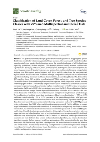
![Remote Sens. 2019, 11, 164 2 of 27
Keywords: tree species; classification; ZiYuan-3; stereo image; machine learning
1. Introduction
A substantial decrease of global forest area from unprecedented human disturbance causes
a huge loss of biodiversity [1]. The expansion of plantations compensates this damage to some
extent. Plantations provide some habitat needs for a subset of animal species and diverse timbers
for human use. Understanding the distribution of plantations is very important in biodiversity
assessment [2], forest biomass prediction [3,4], ecosystem services and biogeochemical cycling [5–7],
and forest resources management [8]. China, as the largest plantation area in the world since 1999 [9],
experienced a dramatic increase from nearly 47 million hectares in 1999 to nearly 70 million hectares in
2014 [10], which requires timely updates of spatial information of forest distribution. Depending on
the geolocations and climate zones in China, the spatial patterns, and types of plantations vary such as
rubbers in a tropical region of south China, eucalyptus in a subtropical region in east and south China,
Chinese fir plantations in the subtropical region, and different kinds of pines (e.g., larch, Chinese pine,
red pine) in north China. Plantations have played more and more important roles in improving
economic conditions for local persons.
Remotely sensed data has long been used for land-cover mapping in large areas due to the
unique characteristics of spectral, temporal, and spatial features and a digital number data format
suitable for computer processing. Satellite data, such as Landsat, have been explored extensively
for land cover mapping, and even individual tree species mapping, because the data are freely
available and contain a broad range of suitable spectral bands [11–14]. Dong et al. [15] combined
multi-temporal Landsat images and PALSAR (Phased Array type L-band Synthetic Aperture Radar)
data to map rubber tree distribution in China’s Hainan Province and achieved an overall accuracy of
92%. Qiao et al. [16] applied time-series normalized difference vegetation index (NDVI) images from
annual Landsat images over 15 years to identify eucalyptus in Guangdong Province and obtained
an accuracy of 91%. In previous research, single-date images were mostly used because of the
difficulty in obtaining images of different seasons due to poor weather conditions, especially in
tropical and subtropical regions [17,18]. Seasonal vegetation information has proven valuable in
improving vegetation classification [19]. In the subtropical Lin’an District mountains, Xi et al. [20]
used multi-temporal Landsat images to extract hickory plantations by developing subpixel indices
from linear spectral mixture analysis. Because of its relatively coarse spatial resolution in Landsat,
accurate mapping of plantation distribution due to a small parch size become a challenge.
In recent years, attention has shifted to using high spatial resolution satellite data for
detailed classification because of its better ability to capture fine characteristics of objects [21–23].
Gomez et al. [17] used QuickBird multispectral and panchromatic images to extract coffee plantations
in NewCaledonia and obtained an accuracy of 96.9%. Cho et al. [24] applied WorldView-2 images to
extract three tree species in South Africa and obtained an accuracy of 89.3%. Wang and Lu [25] used
the expert-rule based approach based on Chinese Gaofen (GF-1) and ZiYuan (ZY-3) satellite images to
successfully map Torrya forest distribution with an overall accuracy of 84.4%. High spatial resolution
data with multi-temporal features are especially valuable for improving vegetation classification
accuracy [19]. Reis and Tasdemir [26] applied QuickBird data during the growing and deciduous
seasons to identify hazelnut in northeastern Turkey and found that accuracy increased by 9% compared
to using single-season data. Li et al. [19] used four-seasonal GF-1 images to map wetland classification
in Hangzhou Way, China using the expert-based approach with an overall classification accuracy of
90.3%. However, processing and analysis of high spatial resolution satellite data also pose challenges
in terms of large file sizes, canopy shadows, and high spectral variation within the forested areas.
The selection of suitable variables from remotely sensed data is one of the critical steps in
improving classification accuracy [27]. Since high spatial resolution data often have limited spectral](data:image/gif;base64,R0lGODlhAQABAIAAAAAAAP///yH5BAEAAAAALAAAAAABAAEAAAIBRAA7)