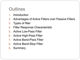
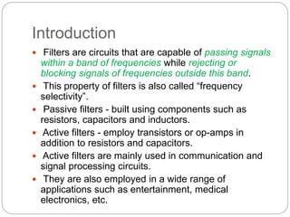
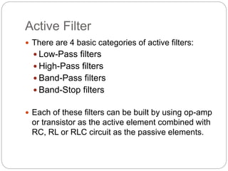
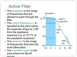
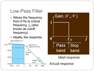
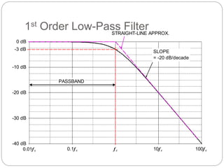
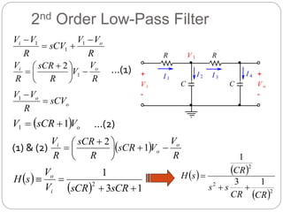
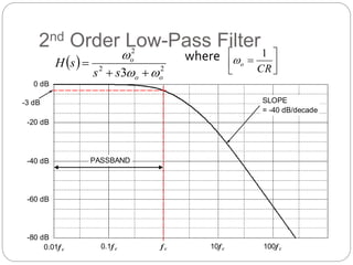
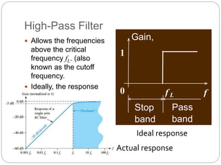
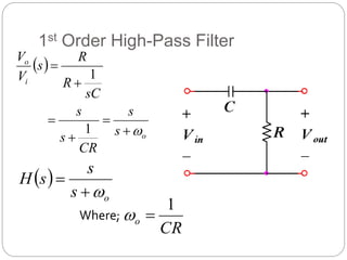
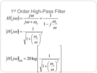
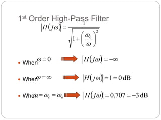
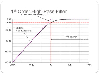
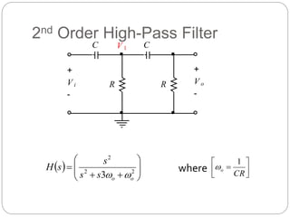
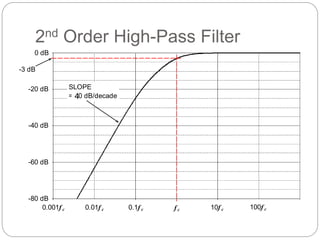
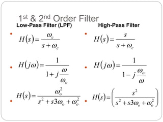
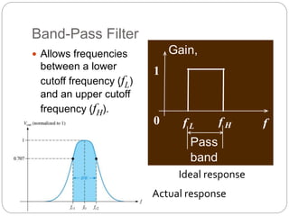
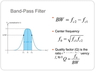
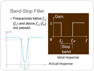
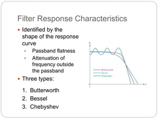
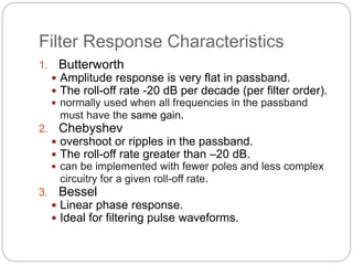
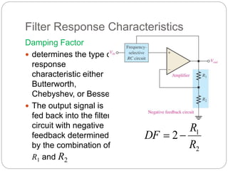
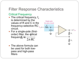
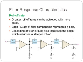
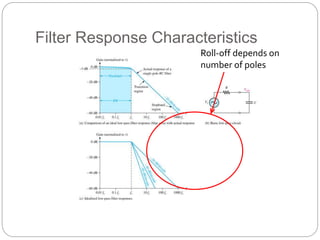
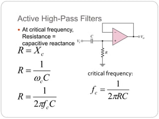
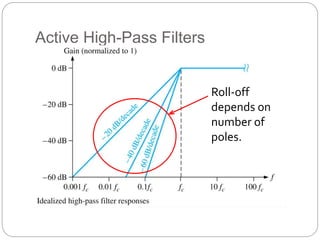
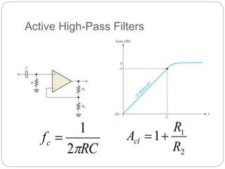
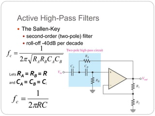
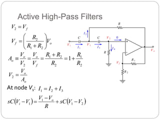
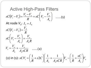
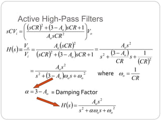
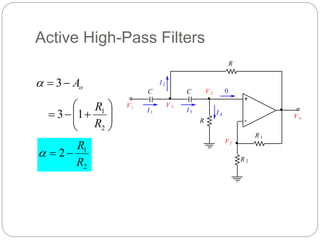
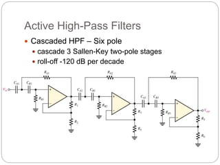
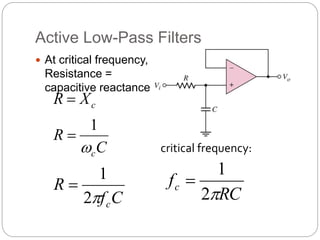
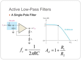
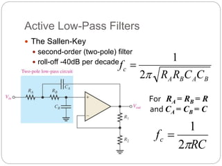
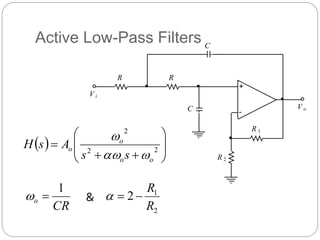
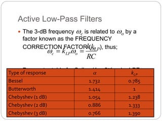
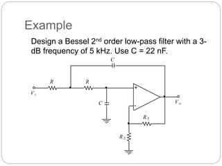
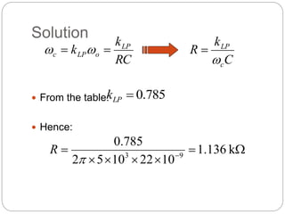
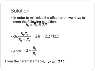
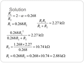
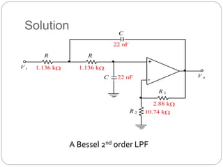
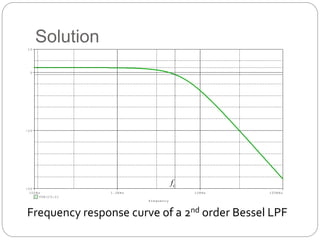
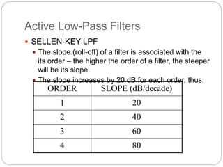
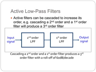
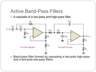
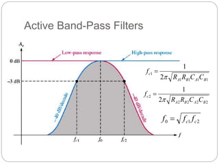
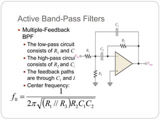
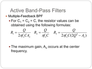
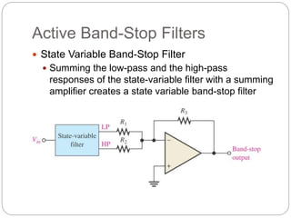
EMT 359/3 – Analog Electronic II
Chapter 5:
Active Filters
Outlines
1. Introduction
2. Advantages of Active Filters over Passive Filters
3. Types of filter
4. Filter Response Characteristic
5. Active Low-Pass Filter
6. Active High-Pass Filter
7. Active Band-Pass Filter
8. Active Band-Stop Filter
9. Summary
Introduction
 Filters are circuits that are capable of passing signals
within a band of frequencies while rejecting or
blocking signals of frequencies outside this band.
 This property of filters is also called “frequency
selectivity”.
 Passive filters - built using components such as
resistors, capacitors and inductors.
 Active filters - employ transistors or op-amps in
addition to resistors and capacitors.
 Active filters are mainly used in communication and
signal processing circuits.
 They are also employed in a wide range of
applications such as entertainment, medical
electronics, etc.
Advantages of Active Filters over Passive
Filters
1. Active filters can be designed to provide
required gain, and hence no attenuation as in
the case of passive filters.
2. No loading problem, because of high input
resistance and low output resistance of op-amp.
3. Active Filters are cost effective as a wide variety
of economical op-amps are available.
Active Filter
 There are 4 basic categories of active filters:
 Low-Pass filters
 High-Pass filters
 Band-Pass filters
 Band-Stop filters
 Each of these filters can be built by using op-amp
or transistor as the active element combined with
RC, RL or RLC circuit as the passive elements.
Active Filter
 The passband is the range
of frequencies that are
allowed to pass through the
filter.
 The critical frequency, fc is
specified at the point where
the response drops by 3 dB
from the passband
response (i.e. to 70.7% of
the passband response)
 The stopband is the range
of frequencies that have the
most attenuation
 The transition region is the
area where the fall-off
Low-Pass Filter
 Allows the frequency
from 0 Hz to critical
frequency, fH (also
known as cutoff
frequency)
 Ideally, the response
drops abruptly at the
critical frequency fH
Ideal response
Actual response
1st Order Low-Pass Filter
   
o
o
i
o
s
CR
s
CR
s
V
V
s
H







1
1
 
o
o
s
s
H




CR
o
1


 
o
o
o
j
j
j
H










1
1
1st Order Low-Pass Filter
 


























2
1
1
log
20
o
dB
j
H



  2
1
1










o
j
H



1st Order Low-Pass Filter
 When
 And
  1
0
1
1
2











o
j
H


0


  dB
0
1
log
20
dB



j
H
1st Order Low-Pass Filter
 When
 And
  707
.
0
1
1
1
1
1
2













o
c
j
H



CR
o
c
1


 


  dB
3
707
.
0
log
20
dB




j
H
CR
c
1

 is known as 3-dB or cutoff
frequency (rad/s)
1st Order Low-Pass Filter
f c
0 dB
-10 dB
-20 dB
-30 dB
-40 dB
-3 dB
PASSBAND
SLOPE
= -20 dB/decade
0.1f c
0.01f c 10f c 100f c
STRAIGHT-LINE APPROX.
2nd Order Low-Pass Filter
R
C
+
V i
-
+
V o
-
R
C
V 1
I 1
I 2 I 3 I 4
R
V
V
sCV
R
V
V o
i 


 1
1
1
R
V
V
R
sCR
R
V o
i






 
 1
2
o
o
sCV
R
V
V


1
…(1)
  o
V
sCR
V 1
1 
 …(2)
(1) & (2)  
R
V
V
sCR
R
sCR
R
V o
o
i







 
 1
2
 
  1
3
1
2




sCR
sCR
V
V
s
H
i
o    
 2
2
2
1
3
1
CR
CR
s
s
CR
s
H



2nd Order Low-Pass Filter
  2
2
2
3 o
o
o
s
s
s
H





 






CR
o
1

where
f c
0.1f c
0.01f c 10f c 100f c
0 dB
-20 dB
-40 dB
-60 dB
-80 dB
-3 dB SLOPE
= -40 dB/decade
PASSBAND
High-Pass Filter
 Allows the frequencies
above the critical
frequency fL. (also
known as the cutoff
frequency.
 Ideally, the response
rises abruptly at the
critical frequency.
0
1
f L f
Gain,
Pass
band
Stop
band
Ideal response
Actual response
1st Order High-Pass Filter
 
o
i
o
s
s
CR
s
s
sC
R
R
s
V
V







1
1
 
o
s
s
s
H



CR
o
1


Where;
1st Order High-Pass Filter
 






o
o j
j
j
j
H




1
1
  2
1
1











o
j
H
 






















2
dB
1
1
log
20



o
j
H
1st Order High-Pass Filter
 When
 When
 When
  2
1
1











o
j
H
0

   


j
H


   dB
0
1


j
H
o
c 

 
   dB
3
707
.
0 



j
H
1st Order High-Pass Filter
f c
0.1f c
0.01f c 10f c 100f c
0 dB
-10 dB
-20 dB
-30 dB
-40 dB
-3 dB
SLOPE
= 20 dB/decade
PASSBAND
STRAIGHT-LINE APPROX.
2nd Order High-Pass Filter
+
V i
-
+
V o
-
R R
V 1
C C
  









 2
2
2
3 o
o
s
s
s
s
H

 






CR
o
1

where
2nd Order High-Pass Filter
f c
0.1f c
0.01f c 10f c 100f c
0.001f c
0 dB
-20 dB
-40 dB
-60 dB
-80 dB
-3 dB
SLOPE
= 20 dB/decade
4
1st & 2nd Order Filter
Low-Pass Filter (LPF) High-Pass Filter






 
c
s
s
s
H



 
c
c
s
s
H




 
o
j
j
H





1
1
 



o
j
j
H


1
1
  2
2
2
3 o
o
o
s
s
s
H





   









 2
2
2
3 o
o
s
s
s
s
H


Band-Pass Filter
 Allows frequencies
between a lower
cutoff frequency (fL)
and an upper cutoff
frequency (fH).
0
1
f L f
Gain,
Pass
band
f H
Ideal response
Actual response
Band-Pass Filter
 Bandwidth (BW)
 Center frequency
 Quality factor (Q) is the
ratio of center frequency
fo to the BW
1
2 c
c f
f
BW 

BW
f
Q 0

2
1
0 c
c f
f
f 
Band-Stop Filter
 Frequencies below fc1
(fL) and above fc2 (fH)
are passed.
0
1
f L f
Gain,
Stop
band
f H
Ideal response
Actual response
Filter Response Characteristics
 Identified by the
shape of the response
curve
• Passband flatness
• Attenuation of
frequency outside
the passband
 Three types:
1. Butterworth
2. Bessel
3. Chebyshev
Filter Response Characteristics
1. Butterworth
 Amplitude response is very flat in passband.
 The roll-off rate -20 dB per decade (per filter order).
 normally used when all frequencies in the passband
must have the same gain.
2. Chebyshev
 overshoot or ripples in the passband.
 The roll-off rate greater than –20 dB.
 can be implemented with fewer poles and less complex
circuitry for a given roll-off rate.
3. Bessel
 Linear phase response.
 Ideal for filtering pulse waveforms.
Filter Response Characteristics
Damping Factor
 determines the type of
response
characteristic either
Butterworth,
Chebyshev, or Bessel.
 The output signal is
fed back into the filter
circuit with negative
feedback determined
by the combination of
R1 and R2
2
1
2
R
R
DF 

Filter Response Characteristics
Critical Frequency
 The critical frequency, fc
is determined by the
values of R and C in the
frequency-selective RC
circuit.
 For a single-pole (first-
order) filter, the critical
frequency is:
 The above formula can
be used for both low-
pass and high-pass
filters
RC
fc

2
1

Filter Response Characteristics
Roll-off rate
 Greater roll-off rates can be achieved with more
poles.
 Each RC set of filter components represents a pole.
 Cascading of filter circuits also increases the poles
which results in a steeper roll-off.
 Each pole represents a –20 dB/decade increase in
roll-off
Filter Response Characteristics
Roll-off depends on
number of poles
Active High-Pass Filters
 At critical frequency,
Resistance =
capacitive reactance
c
X
R 
C
f
R
c

2
1

C
R
c

1
 critical frequency:
RC
fc

2
1

Active High-Pass Filters
Roll-off
depends on
number of
poles.
Active High-Pass Filters
 A Single-Pole Filter
RC
fc

2
1

2
1
1
R
R
Acl 

Active High-Pass Filters
 The Sallen-Key
 second-order (two-pole) filter
 roll-off -40dB per decade
RC
fc

2
1

Lets RA = RB = R
and CA = CB = C;
B
A
B
A
c
C
C
R
R
f

2
1

Active High-Pass Filters
C C
R
R
R 1
R 2
+
-
V o
V i
V f
V 1
V 2
I 1
I 2
I 3 I 4
0
f
V
V 
2
o
f V
R
R
R
V 









2
1
2
2
1
2
2
1
2
1
R
R
R
R
R
V
V
V
V
A
f
o
o
o 





o
o
A
V
V 
2
3
2
1 I
I
I 

   
2
1
1
1 V
V
sC
R
V
V
V
V
sC o
i 




At node V1:
Active High-Pass Filters
  












o
o
o
i
A
V
V
sC
R
V
V
V
V
sC 1
1
1 ……(1)
4
3 I
I 
 
R
V
V
V
sC 2
2
1 

R
A
V
A
V
V
sC
o
o
o
o










1
sCR
A
V
A
V
V
o
o
o
o


1 ……(2)
At node V2:
(2) in (1): o
o
o
o
o
i V
A
sC
R
V
sCR
A
A
C
s
R
sCV 


























1
1
1
2
1
Active High-Pass Filters
   
    1
3
2
2





sCR
A
sCR
sCR
A
V
V
s
H
o
o
i
o
   
o
o
o
i V
sCR
A
sCR
A
sCR
sCV 






 


 2
2
1
3
 
 2
2
2
1
3
CR
s
CR
A
s
s
A
o
o




  2
2
2
3 o
o
o
o
s
A
s
s
A

 



CR
o
1


where
o
A

 3

  2
2
2
o
o
o
s
s
s
A
s
H

 


= Damping Factor
Active High-Pass Filters
C C
R
R
R 1
R 2
+
-
V o
V i
V f
V 1
V 2
I 1
I 2
I 3 I 4
0
o
A

 3












2
1
1
3
R
R
2
1
2
R
R



Active High-Pass Filters
 Cascaded HPF – Six pole
 cascade 3 Sallen-Key two-pole stages
 roll-off -120 dB per decade
Active Low-Pass Filters
 At critical frequency,
Resistance =
capacitive reactance
c
X
R 
C
f
R
c

2
1

C
R
c

1

critical frequency:
RC
fc

2
1

Active Low-Pass Filters
 A Single-Pole Filter
2
1
1
R
R
Acl 

RC
fc

2
1

Active Low-Pass Filters
 The Sallen-Key
 second-order (two-pole) filter
 roll-off -40dB per decade
RC
fc

2
1

For RA = RB = R
and CA = CB = C
B
A
B
A
c
C
C
R
R
f

2
1

Active Low-Pass Filters
C
C
R R
R 1
R 2
+
-
V i
V o
  









 2
2
2
o
o
o
o
s
s
A
s
H



CR
o
1


2
1
2
R
R



&
Active Low-Pass Filters
 The 3-dB frequency c is related to o by a
factor known as the FREQUENCY
CORRECTION FACTOR (kLP), thus;
 Parameter table for Sellen-Key 2nd order LPF
RC
k
k LP
o
LP
c 
 

Type of response  kLP
Bessel 1.732 0.785
Butterworth 1.414 1
Chebyshev (1 dB) 1.054 1.238
Chebyshev (2 dB) 0.886 1.333
Chebyshev (3 dB) 0.766 1.390
Example
Design a Bessel 2nd order low-pass filter with a 3-
dB frequency of 5 kHz. Use C = 22 nF.
C
C
R R
R 1
R 2
+
-
V i
V o
Solution
 From the table:
 Hence:
RC
k
k LP
o
LP
c 
 

C
k
R
c
LP


785
.
0

LP
k






 
k
136
.
1
10
22
10
5
2
785
.
0
9
3

R
Solution
 In order to minimize the offset error, we have to
meet the following condition:
 Or;
 And:
R
R
R 2
// 2
1 




k
27
.
2
2
2
1
2
1
R
R
R
R
R
2
1
2
R
R



From the parameter table; 732
.
1


Solution
268
.
0
2
2
1


 
R
R
2
1 268
.
0 R
R  


k
27
.
2
2
1
2
1
R
R
R
R



k
27
.
2
268
.
0
268
.
0
2
2
2
2
R
R
R



 k
10.74
268
.
0
27
.
2
268
.
1
2
R




 k
88
.
2
74
.
10
268
.
0
268
.
0 2
1 R
R
Solution
C
C
R R
R 1
R 2
+
-
V i
V o
1.136 k 1.136 k
22 nF
22 nF
2.88 k
10.74 k
A Bessel 2nd order LPF
Solution
Frequency response curve of a 2nd order Bessel LPF
Frequency
100Hz 1.0KHz 10KHz 100KHz
VDB(C5:2)
-50
-25
0
10
fc
Example
1. Determine critical frequency
2. Set the value of R1 for Butterworth response
Solution
1. Critical frequency
2. Butterworth response, R1/R2 = 0.586
kHz
23
.
7
2
1


RC
fc

2
1 586
.
0 R
R 
kΩ
586
1 
R
Active Low-Pass Filters
 Cascaded LPF – Three-pole
 cascade two-pole and single-pole
 roll-off -60dB per decade
Active Low-Pass Filters
 Cascaded LPF – Four pole
 cascade two-pole and two-pole
 roll-off -80dB per decade
Example
Determine the capacitance values required to
produce a critical frequency of 2680 Hz if all
resistors in RC low pass circuit is 1.8 k
Solution
RC
fc

2
1

μF
033
.
0
2
1


R
f
C
c

μF
033
.
0
2
2
1
1 


 B
A
B
A C
C
C
C
Active Low-Pass Filters
 SELLEN-KEY LPF
 The slope (roll-off) of a filter is associated with the
its order – the higher the order of a filter, the steeper
will be its slope.
 The slope increases by 20 dB for each order, thus;
ORDER SLOPE (dB/decade)
1 20
2 40
3 60
4 80
Active Low-Pass Filters
 Active filters can be cascaded to increase its
order, e.g. cascading a 2nd order and a 1st order
filter will produce a 3rd order filter
2nd order
LPF
1st order
LPF
Input
signal
Output
signal
Cascading a 2nd order and a 1st order filter produces a 3rd
order filter with a roll-off of 60dB/decade
Active Band-Pass Filters
 A cascade of a low-pass and high-pass filter
 Band-pass filter formed by cascading a two-pole high-pass
and a two-pole low-pass filters
Active Band-Pass Filters
2
1
0 c
c f
f
f 
1
1
1
1
1
2
1
B
A
B
A
c
C
C
R
R
f


2
2
2
2
2
2
1
B
A
B
A
c
C
C
R
R
f


Active Band-Pass Filters
 Multiple-Feedback
BPF
 The low-pass circuit
consists of R1 and C1.
 The high-pass circuit
consists of R2 and C2.
 The feedback paths
are through C1 and R2.
 Center frequency:
  2
1
2
3
1
0
//
2
1
C
C
R
R
R
f


Active Band-Pass Filters
 Multiple-Feedback BPF
 For C1 = C2 = C, the resistor values can be
obtained using the following formulas:
 The maximum gain, Ao occurs at the center
frequency.
o
oCA
f
Q
R

2
1 
C
f
Q
R
o


2
)
2
(
2 2
3
o
o A
Q
C
f
Q
R



Active Band-Pass Filters
 State-Variable BPF
 It consists of a summing amplifier and two integrators.
 It has outputs for low-pass, high-pass, and band-pass.
 The center frequency is set by the integrator RC
circuits.
 R5 and R6 set the Q (bandwidth). 








 1
3
1
6
5
R
R
Q
Active Band-Pass Filters
 The band-pass output peaks sharply the center
frequency giving it a high Q.
Active Band-Pass Filters
 Biquad Filter
 contains an integrator, followed by an inverting
amplifier, and then an integrator.
 In a biquad filter, the bandwidth is independent
and the Q is dependent on the critical frequency.
Active Band-Stop Filters
 The BSF is opposite of BPF in that it blocks a
specific band of frequencies.
 The multiple-feedback design is similar to a BPF
with exception of the placement of R3 and the
addition of R4
Active Band-Stop Filters
 State Variable Band-Stop Filter
 Summing the low-pass and the high-pass
responses of the state-variable filter with a summing
amplifier creates a state variable band-stop filter
Summary
 The bandwidth of a low-pass filter is the same as
the upper critical frequency.
 The bandwidth of a high-pass filter extends from
the lower critical frequency up to the inherent
limits of the circuit.
 The band-pass passes frequencies between the
lower critical frequency and the upper critical
frequency.
 A band-stop filter rejects frequencies within the
upper critical frequency and upper critical
frequency.
Summary
 The Butterworth filter response is very flat and
has a roll-off rate of –20 dB.
 The Chebyshev filter response has ripples and
overshoot in the passband but can have roll-off
rates greater than –20 dB.
 The Bessel response exhibits a linear phase
characteristic, and filters with the Bessel
response are better for filtering pulse waveforms.
Summary
 A filter pole consists of one RC circuit. Each pole
doubles the roll-off rate.
 The Q of a filter indicates a band-pass filter’s
selectivity. The higher the Q the narrower the
bandwidth.
 The damping factor determines the filter response
characteristic.

16971168.ppt

  • 1.
    EMT 359/3 –Analog Electronic II Chapter 5: Active Filters
  • 2.
    Outlines 1. Introduction 2. Advantagesof Active Filters over Passive Filters 3. Types of filter 4. Filter Response Characteristic 5. Active Low-Pass Filter 6. Active High-Pass Filter 7. Active Band-Pass Filter 8. Active Band-Stop Filter 9. Summary
  • 3.
    Introduction  Filters arecircuits that are capable of passing signals within a band of frequencies while rejecting or blocking signals of frequencies outside this band.  This property of filters is also called “frequency selectivity”.  Passive filters - built using components such as resistors, capacitors and inductors.  Active filters - employ transistors or op-amps in addition to resistors and capacitors.  Active filters are mainly used in communication and signal processing circuits.  They are also employed in a wide range of applications such as entertainment, medical electronics, etc.
  • 4.
    Advantages of ActiveFilters over Passive Filters 1. Active filters can be designed to provide required gain, and hence no attenuation as in the case of passive filters. 2. No loading problem, because of high input resistance and low output resistance of op-amp. 3. Active Filters are cost effective as a wide variety of economical op-amps are available.
  • 5.
    Active Filter  Thereare 4 basic categories of active filters:  Low-Pass filters  High-Pass filters  Band-Pass filters  Band-Stop filters  Each of these filters can be built by using op-amp or transistor as the active element combined with RC, RL or RLC circuit as the passive elements.
  • 6.
    Active Filter  Thepassband is the range of frequencies that are allowed to pass through the filter.  The critical frequency, fc is specified at the point where the response drops by 3 dB from the passband response (i.e. to 70.7% of the passband response)  The stopband is the range of frequencies that have the most attenuation  The transition region is the area where the fall-off
  • 7.
    Low-Pass Filter  Allowsthe frequency from 0 Hz to critical frequency, fH (also known as cutoff frequency)  Ideally, the response drops abruptly at the critical frequency fH Ideal response Actual response
  • 8.
    1st Order Low-PassFilter     o o i o s CR s CR s V V s H        1 1   o o s s H     CR o 1     o o o j j j H           1 1
  • 9.
    1st Order Low-PassFilter                             2 1 1 log 20 o dB j H      2 1 1           o j H   
  • 10.
    1st Order Low-PassFilter  When  And   1 0 1 1 2            o j H   0     dB 0 1 log 20 dB    j H
  • 11.
    1st Order Low-PassFilter  When  And   707 . 0 1 1 1 1 1 2              o c j H    CR o c 1         dB 3 707 . 0 log 20 dB     j H CR c 1   is known as 3-dB or cutoff frequency (rad/s)
  • 12.
    1st Order Low-PassFilter f c 0 dB -10 dB -20 dB -30 dB -40 dB -3 dB PASSBAND SLOPE = -20 dB/decade 0.1f c 0.01f c 10f c 100f c STRAIGHT-LINE APPROX.
  • 13.
    2nd Order Low-PassFilter R C + V i - + V o - R C V 1 I 1 I 2 I 3 I 4 R V V sCV R V V o i     1 1 1 R V V R sCR R V o i          1 2 o o sCV R V V   1 …(1)   o V sCR V 1 1   …(2) (1) & (2)   R V V sCR R sCR R V o o i           1 2     1 3 1 2     sCR sCR V V s H i o      2 2 2 1 3 1 CR CR s s CR s H   
  • 14.
    2nd Order Low-PassFilter   2 2 2 3 o o o s s s H              CR o 1  where f c 0.1f c 0.01f c 10f c 100f c 0 dB -20 dB -40 dB -60 dB -80 dB -3 dB SLOPE = -40 dB/decade PASSBAND
  • 15.
    High-Pass Filter  Allowsthe frequencies above the critical frequency fL. (also known as the cutoff frequency.  Ideally, the response rises abruptly at the critical frequency. 0 1 f L f Gain, Pass band Stop band Ideal response Actual response
  • 16.
    1st Order High-PassFilter   o i o s s CR s s sC R R s V V        1 1   o s s s H    CR o 1   Where;
  • 17.
    1st Order High-PassFilter         o o j j j j H     1 1   2 1 1            o j H                         2 dB 1 1 log 20    o j H
  • 18.
    1st Order High-PassFilter  When  When  When   2 1 1            o j H 0        j H      dB 0 1   j H o c        dB 3 707 . 0     j H
  • 19.
    1st Order High-PassFilter f c 0.1f c 0.01f c 10f c 100f c 0 dB -10 dB -20 dB -30 dB -40 dB -3 dB SLOPE = 20 dB/decade PASSBAND STRAIGHT-LINE APPROX.
  • 20.
    2nd Order High-PassFilter + V i - + V o - R R V 1 C C              2 2 2 3 o o s s s s H          CR o 1  where
  • 21.
    2nd Order High-PassFilter f c 0.1f c 0.01f c 10f c 100f c 0.001f c 0 dB -20 dB -40 dB -60 dB -80 dB -3 dB SLOPE = 20 dB/decade 4
  • 22.
    1st & 2ndOrder Filter Low-Pass Filter (LPF) High-Pass Filter         c s s s H      c c s s H       o j j H      1 1      o j j H   1 1   2 2 2 3 o o o s s s H                    2 2 2 3 o o s s s s H  
  • 23.
    Band-Pass Filter  Allowsfrequencies between a lower cutoff frequency (fL) and an upper cutoff frequency (fH). 0 1 f L f Gain, Pass band f H Ideal response Actual response
  • 24.
    Band-Pass Filter  Bandwidth(BW)  Center frequency  Quality factor (Q) is the ratio of center frequency fo to the BW 1 2 c c f f BW   BW f Q 0  2 1 0 c c f f f 
  • 25.
    Band-Stop Filter  Frequenciesbelow fc1 (fL) and above fc2 (fH) are passed. 0 1 f L f Gain, Stop band f H Ideal response Actual response
  • 26.
    Filter Response Characteristics Identified by the shape of the response curve • Passband flatness • Attenuation of frequency outside the passband  Three types: 1. Butterworth 2. Bessel 3. Chebyshev
  • 27.
    Filter Response Characteristics 1.Butterworth  Amplitude response is very flat in passband.  The roll-off rate -20 dB per decade (per filter order).  normally used when all frequencies in the passband must have the same gain. 2. Chebyshev  overshoot or ripples in the passband.  The roll-off rate greater than –20 dB.  can be implemented with fewer poles and less complex circuitry for a given roll-off rate. 3. Bessel  Linear phase response.  Ideal for filtering pulse waveforms.
  • 28.
    Filter Response Characteristics DampingFactor  determines the type of response characteristic either Butterworth, Chebyshev, or Bessel.  The output signal is fed back into the filter circuit with negative feedback determined by the combination of R1 and R2 2 1 2 R R DF  
  • 29.
    Filter Response Characteristics CriticalFrequency  The critical frequency, fc is determined by the values of R and C in the frequency-selective RC circuit.  For a single-pole (first- order) filter, the critical frequency is:  The above formula can be used for both low- pass and high-pass filters RC fc  2 1 
  • 30.
    Filter Response Characteristics Roll-offrate  Greater roll-off rates can be achieved with more poles.  Each RC set of filter components represents a pole.  Cascading of filter circuits also increases the poles which results in a steeper roll-off.  Each pole represents a –20 dB/decade increase in roll-off
  • 31.
    Filter Response Characteristics Roll-offdepends on number of poles
  • 32.
    Active High-Pass Filters At critical frequency, Resistance = capacitive reactance c X R  C f R c  2 1  C R c  1  critical frequency: RC fc  2 1 
  • 33.
  • 34.
    Active High-Pass Filters A Single-Pole Filter RC fc  2 1  2 1 1 R R Acl  
  • 35.
    Active High-Pass Filters The Sallen-Key  second-order (two-pole) filter  roll-off -40dB per decade RC fc  2 1  Lets RA = RB = R and CA = CB = C; B A B A c C C R R f  2 1 
  • 36.
    Active High-Pass Filters CC R R R 1 R 2 + - V o V i V f V 1 V 2 I 1 I 2 I 3 I 4 0 f V V  2 o f V R R R V           2 1 2 2 1 2 2 1 2 1 R R R R R V V V V A f o o o       o o A V V  2 3 2 1 I I I       2 1 1 1 V V sC R V V V V sC o i      At node V1:
  • 37.
    Active High-Pass Filters               o o o i A V V sC R V V V V sC 1 1 1 ……(1) 4 3 I I    R V V V sC 2 2 1   R A V A V V sC o o o o           1 sCR A V A V V o o o o   1 ……(2) At node V2: (2) in (1): o o o o o i V A sC R V sCR A A C s R sCV                            1 1 1 2 1
  • 38.
    Active High-Pass Filters        1 3 2 2      sCR A sCR sCR A V V s H o o i o     o o o i V sCR A sCR A sCR sCV             2 2 1 3    2 2 2 1 3 CR s CR A s s A o o       2 2 2 3 o o o o s A s s A       CR o 1   where o A   3    2 2 2 o o o s s s A s H      = Damping Factor
  • 39.
    Active High-Pass Filters CC R R R 1 R 2 + - V o V i V f V 1 V 2 I 1 I 2 I 3 I 4 0 o A   3             2 1 1 3 R R 2 1 2 R R   
  • 40.
    Active High-Pass Filters Cascaded HPF – Six pole  cascade 3 Sallen-Key two-pole stages  roll-off -120 dB per decade
  • 41.
    Active Low-Pass Filters At critical frequency, Resistance = capacitive reactance c X R  C f R c  2 1  C R c  1  critical frequency: RC fc  2 1 
  • 42.
    Active Low-Pass Filters A Single-Pole Filter 2 1 1 R R Acl   RC fc  2 1 
  • 43.
    Active Low-Pass Filters The Sallen-Key  second-order (two-pole) filter  roll-off -40dB per decade RC fc  2 1  For RA = RB = R and CA = CB = C B A B A c C C R R f  2 1 
  • 44.
    Active Low-Pass Filters C C RR R 1 R 2 + - V i V o              2 2 2 o o o o s s A s H    CR o 1   2 1 2 R R    &
  • 45.
    Active Low-Pass Filters The 3-dB frequency c is related to o by a factor known as the FREQUENCY CORRECTION FACTOR (kLP), thus;  Parameter table for Sellen-Key 2nd order LPF RC k k LP o LP c     Type of response  kLP Bessel 1.732 0.785 Butterworth 1.414 1 Chebyshev (1 dB) 1.054 1.238 Chebyshev (2 dB) 0.886 1.333 Chebyshev (3 dB) 0.766 1.390
  • 46.
    Example Design a Bessel2nd order low-pass filter with a 3- dB frequency of 5 kHz. Use C = 22 nF. C C R R R 1 R 2 + - V i V o
  • 47.
    Solution  From thetable:  Hence: RC k k LP o LP c     C k R c LP   785 . 0  LP k         k 136 . 1 10 22 10 5 2 785 . 0 9 3  R
  • 48.
    Solution  In orderto minimize the offset error, we have to meet the following condition:  Or;  And: R R R 2 // 2 1      k 27 . 2 2 2 1 2 1 R R R R R 2 1 2 R R    From the parameter table; 732 . 1  
  • 49.
    Solution 268 . 0 2 2 1     R R 2 1 268 . 0R R     k 27 . 2 2 1 2 1 R R R R    k 27 . 2 268 . 0 268 . 0 2 2 2 2 R R R     k 10.74 268 . 0 27 . 2 268 . 1 2 R      k 88 . 2 74 . 10 268 . 0 268 . 0 2 1 R R
  • 50.
    Solution C C R R R 1 R2 + - V i V o 1.136 k 1.136 k 22 nF 22 nF 2.88 k 10.74 k A Bessel 2nd order LPF
  • 51.
    Solution Frequency response curveof a 2nd order Bessel LPF Frequency 100Hz 1.0KHz 10KHz 100KHz VDB(C5:2) -50 -25 0 10 fc
  • 52.
    Example 1. Determine criticalfrequency 2. Set the value of R1 for Butterworth response
  • 53.
    Solution 1. Critical frequency 2.Butterworth response, R1/R2 = 0.586 kHz 23 . 7 2 1   RC fc  2 1 586 . 0 R R  kΩ 586 1  R
  • 54.
    Active Low-Pass Filters Cascaded LPF – Three-pole  cascade two-pole and single-pole  roll-off -60dB per decade
  • 55.
    Active Low-Pass Filters Cascaded LPF – Four pole  cascade two-pole and two-pole  roll-off -80dB per decade
  • 56.
    Example Determine the capacitancevalues required to produce a critical frequency of 2680 Hz if all resistors in RC low pass circuit is 1.8 k
  • 57.
  • 58.
    Active Low-Pass Filters SELLEN-KEY LPF  The slope (roll-off) of a filter is associated with the its order – the higher the order of a filter, the steeper will be its slope.  The slope increases by 20 dB for each order, thus; ORDER SLOPE (dB/decade) 1 20 2 40 3 60 4 80
  • 59.
    Active Low-Pass Filters Active filters can be cascaded to increase its order, e.g. cascading a 2nd order and a 1st order filter will produce a 3rd order filter 2nd order LPF 1st order LPF Input signal Output signal Cascading a 2nd order and a 1st order filter produces a 3rd order filter with a roll-off of 60dB/decade
  • 60.
    Active Band-Pass Filters A cascade of a low-pass and high-pass filter  Band-pass filter formed by cascading a two-pole high-pass and a two-pole low-pass filters
  • 61.
    Active Band-Pass Filters 2 1 0c c f f f  1 1 1 1 1 2 1 B A B A c C C R R f   2 2 2 2 2 2 1 B A B A c C C R R f  
  • 62.
    Active Band-Pass Filters Multiple-Feedback BPF  The low-pass circuit consists of R1 and C1.  The high-pass circuit consists of R2 and C2.  The feedback paths are through C1 and R2.  Center frequency:   2 1 2 3 1 0 // 2 1 C C R R R f  
  • 63.
    Active Band-Pass Filters Multiple-Feedback BPF  For C1 = C2 = C, the resistor values can be obtained using the following formulas:  The maximum gain, Ao occurs at the center frequency. o oCA f Q R  2 1  C f Q R o   2 ) 2 ( 2 2 3 o o A Q C f Q R   
  • 64.
    Active Band-Pass Filters State-Variable BPF  It consists of a summing amplifier and two integrators.  It has outputs for low-pass, high-pass, and band-pass.  The center frequency is set by the integrator RC circuits.  R5 and R6 set the Q (bandwidth).           1 3 1 6 5 R R Q
  • 65.
    Active Band-Pass Filters The band-pass output peaks sharply the center frequency giving it a high Q.
  • 66.
    Active Band-Pass Filters Biquad Filter  contains an integrator, followed by an inverting amplifier, and then an integrator.  In a biquad filter, the bandwidth is independent and the Q is dependent on the critical frequency.
  • 67.
    Active Band-Stop Filters The BSF is opposite of BPF in that it blocks a specific band of frequencies.  The multiple-feedback design is similar to a BPF with exception of the placement of R3 and the addition of R4
  • 68.
    Active Band-Stop Filters State Variable Band-Stop Filter  Summing the low-pass and the high-pass responses of the state-variable filter with a summing amplifier creates a state variable band-stop filter
  • 69.
    Summary  The bandwidthof a low-pass filter is the same as the upper critical frequency.  The bandwidth of a high-pass filter extends from the lower critical frequency up to the inherent limits of the circuit.  The band-pass passes frequencies between the lower critical frequency and the upper critical frequency.  A band-stop filter rejects frequencies within the upper critical frequency and upper critical frequency.
  • 70.
    Summary  The Butterworthfilter response is very flat and has a roll-off rate of –20 dB.  The Chebyshev filter response has ripples and overshoot in the passband but can have roll-off rates greater than –20 dB.  The Bessel response exhibits a linear phase characteristic, and filters with the Bessel response are better for filtering pulse waveforms.
  • 71.
    Summary  A filterpole consists of one RC circuit. Each pole doubles the roll-off rate.  The Q of a filter indicates a band-pass filter’s selectivity. The higher the Q the narrower the bandwidth.  The damping factor determines the filter response characteristic.