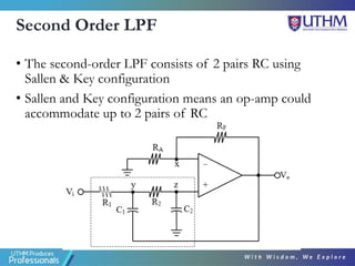
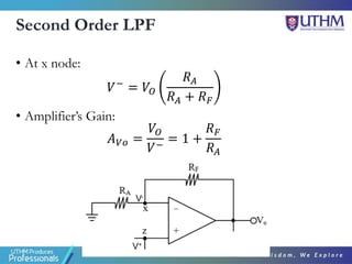
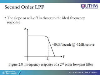
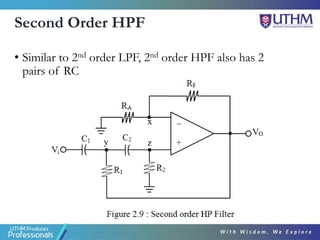
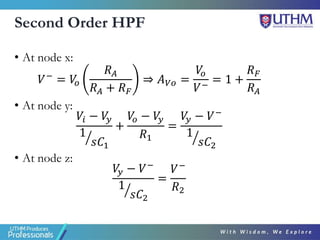
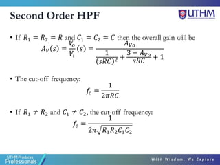
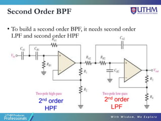
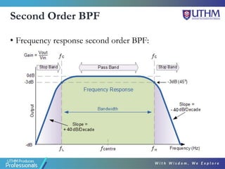
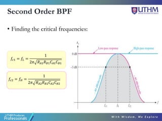
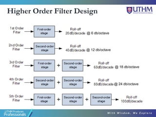
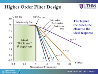
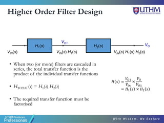
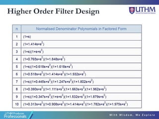
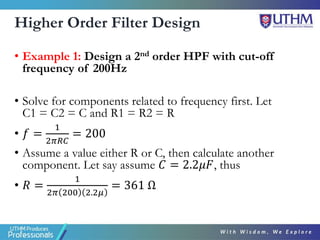
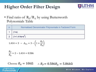
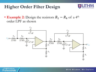
BEJ 30403
ELECTRONIC CIRCUIT
ANALYSIS AND DESIGN
Chapter 2 Active Filter
Part III
Dr. Rahmat Sanudin
Department of Electronic Engineering
Faculty of Electrical and Electronic Engineering
Outline
•Second Order Low Pass Filter
•Second Order High Pass Filter
•Second Order Band-Pass Filter
•Higher Order Filter Design
Second Order LPF
• The second-order LPF consists of 2 pairs RC using
Sallen & Key configuration
• Sallen and Key configuration means an op-amp could
accommodate up to 2 pairs of RC
Second Order LPF
• At x node:
𝑉− = 𝑉𝑂
𝑅𝐴
𝑅𝐴 + 𝑅𝐹
• Amplifier’s Gain:
𝐴𝑉𝑜 =
𝑉𝑂
𝑉−
= 1 +
𝑅𝐹
𝑅𝐴
V-
V+
Second Order LPF
• At y node:
𝑉𝑖 − 𝑉
𝑦
𝑅1
+ 𝑉𝑂 − 𝑉
𝑦 𝑗𝜔𝐶1 =
𝑉
𝑦 − 𝑉−
𝑅2
• Substitute 𝑗𝜔 = 𝑠
𝑉𝑖 − 𝑉
𝑦
𝑅1
+ 𝑉𝑂 − 𝑉
𝑦 𝑠𝐶1 =
𝑉
𝑦 − 𝑉−
𝑅2
V-
Vo
Second Order LPF
• At z node:
𝑉
𝑦 − 𝑉−
𝑅2
=
𝑉−
ൗ
1
𝑗𝜔𝐶2
𝑉
𝑦 − 𝑉−
𝑅2
= 𝑗𝜔𝐶2𝑉−
• Substitute 𝑗𝜔 = 𝑠
𝑉
𝑦 − 𝑉−
𝑅2
= 𝑠𝐶2𝑉−
V-
Vo
Second Order LPF
If R1 = R2 = R and C1 = C2 = C
simplifying all those equations, the overall gain will be:
𝐴𝑉(𝑠) =
𝑉𝑂
𝑉𝑖
(𝑠) =
𝐴𝑉𝑂
(𝑅𝐶𝑠)2 + (3 − 𝐴𝑉𝑂)𝑅𝐶𝑠 + 1
𝐴𝑉𝑜 =
𝑉𝑂
𝑉−
= 1 +
𝑅𝐹
𝑅𝐴
𝑉𝑖 − 𝑉
𝑦
𝑅1
+ 𝑉𝑂 − 𝑉
𝑦 𝑠𝐶1 =
𝑉
𝑦 − 𝑉−
𝑅2
𝑉
𝑦 − 𝑉−
𝑅2
= 𝑠𝐶2𝑉−
Second Order LPF
• With R1 = R2 = R and C1 = C2 = C, the overall gain :
𝐴𝑉(𝑠) =
𝑉𝑂
𝑉𝑖
(𝑠) =
𝐴𝑉𝑂
(𝑅𝐶𝑠)2 + (3 − 𝐴𝑉𝑂)𝑅𝐶𝑠 + 1
• The cut-off frequency:
𝑓𝑐 =
1
2𝜋𝑅𝐶
• If R1 ≠ R2 and C1 ≠ C2 :
𝑓𝑐 =
1
2𝜋 𝑅1𝐶1𝑅2𝐶2
Second Order LPF
• The slope or roll-off is closer to the ideal frequency
response
Second Order HPF
• Similar to 2nd order LPF, 2nd order HPF also has 2
pairs of RC
Second Order HPF
• At node x:
𝑉− = 𝑉
𝑜
𝑅𝐴
𝑅𝐴 + 𝑅𝐹
⇒ 𝐴𝑉𝑜 =
𝑉
𝑜
𝑉−
= 1 +
𝑅𝐹
𝑅𝐴
• At node y:
𝑉𝑖 − 𝑉
𝑦
ൗ
1
𝑠𝐶1
+
𝑉
𝑜 − 𝑉
𝑦
𝑅1
=
𝑉
𝑦 − 𝑉−
ൗ
1
𝑠𝐶2
• At node z:
𝑉
𝑦 − 𝑉−
ൗ
1
𝑠𝐶2
=
𝑉−
𝑅2
Second Order HPF
• If 𝑅1 = 𝑅2 = 𝑅 and 𝐶1 = 𝐶2 = 𝐶 then the overall gain will be
𝐴𝑉 𝑠 =
𝑉
𝑜
𝑉𝑖
𝑠 =
𝐴𝑉𝑜
1
𝑠𝑅𝐶 2 +
3 − 𝐴𝑉𝑜
𝑠𝑅𝐶
+ 1
• The cut-off frequency:
𝑓𝑐 =
1
2𝜋𝑅𝐶
• If 𝑅1 ≠ 𝑅2 and 𝐶1 ≠ 𝐶2, the cut-off frequency:
𝑓𝑐 =
1
2𝜋 𝑅1𝑅2𝐶1𝐶2
Second Order BPF
• To build a second order BPF, it needs second order
LPF and second order HPF
2nd order
LPF
2nd order
HPF
Second Order BPF
• Frequency response second order BPF:
Second Order BPF
• Finding the critical frequencies:
𝑓𝑐1 = 𝑓𝐿 =
1
2𝜋 𝑅𝐴1𝑅𝐵1𝐶𝐴1𝐶𝐵1
𝑓𝑐2 = 𝑓𝐻 =
1
2𝜋 𝑅𝐴2𝑅𝐵2𝐶𝐴2𝐶𝐵2
Second Order BPF
• Centre frequency (f0): The geometric mean
(average) of the cutoff frequencies
• Quality factor (Q): The ratio of filter centre
frequency (f0 = fc) to filter bandwidth (BW)
𝑄 =
𝑓0
𝐵𝑊
=
𝑓0
𝑓𝐻 − 𝑓𝐿
𝑓0 = 𝑓𝑐1𝑓𝑐2 = 𝑓𝐿𝑓𝐻
Higher Order Filter Design
@ 6 db/octave
@ 12 db/octave
@ 18 db/octave
@ 24 db/octave
Higher Order Filter Design
The higher
the order, the
closer to the
ideal response
Higher Order Filter Design
• When two (or more) filters are cascaded in
series, the total transfer function is the
product of the individual transfer functions
• HTOTAL(s) = H1(s) H2(s)
• The required transfer function must be
factorised
H1(s) H2(s)
VIN(s) VIN(s) H1(s) VIN(s) H1(s) H2(s)
𝐻 𝑠 =
𝑉𝑂1
𝑉𝑖𝑛
×
𝑉𝑂
𝑉𝑂1
= 𝐻1 𝑠 × 𝐻2 𝑠
VO1
VO
Higher Order Filter Design
• In filter design, a term known “Butterworth
Polynomials” has been formulated to aid the process
of the design
• These polynomials is useful to determine the required
values of resistors related to filter gain
• The list of “Butterworth Polynomials” is given in
table in the next slide
Higher Order Filter Design
• In higher order filter design, the Sallen & Key
configuration is normally used
• The Sallen and Key configuration realises a two-pole
filter section using a single op-amp
• Synthesis by sections creates higher order filters by
cascading first and second order sections
• Under ideal assumptions, the order of the sections is
irrelevant
• Practically, dynamic range considerations decide the
order of the sections
Higher Order Filter Design
• To get the highest maximum input signal range:
• Sections with the largest damping ratio (lowest Q) should come
first
• Resonant sections with low damping ratios come last, possibly
susceptible to noise
• To get the lowest output noise:
• Highest gain sections (i.e. most resonant) should come first
• Subsequent sections attenuate noise
• What is the best order ?
• It depends on the required specification
Higher Order Filter Design
• Example 1: Design a 2nd order HPF with cut-off
frequency of 200Hz
• Solve for components related to frequency first. Let
C1 = C2 = C and R1 = R2 = R
• 𝑓 =
1
2𝜋𝑅𝐶
= 200
• Assume a value either R or C, then calculate another
component. Let say assume 𝐶 = 2.2𝜇𝐹, thus
• 𝑅 =
1
2𝜋 200 2.2𝜇
= 361 Ω
Higher Order Filter Design
• Find ratio of RF/RA by using Butterworth
Polynomials Table
𝑅𝐹
𝑅𝐴
= 2 − 1.414 = 0.586
1.414 = 3 − 𝐴𝑉𝑜 = 3 − 1 +
𝑅𝐹
𝑅𝐴
Choose 𝑅𝐴 = 10𝑘Ω ∴ 𝑅𝐹= 0.586𝑅𝐴 = 5.86𝑘Ω
Higher Order Filter Design
• Example 2: Design the resistors 𝑅1 − 𝑅4 of a 4th
order LPF as shown
+
+
–
–
R
R
1
3
R
R
2
4
R
R
B1
B2
R
R
A1
A2
C
C
A1
A2
C
C
B1
B2
Vin
Vout
22 kW
22 kW
22 kW
22 kW
4.7 nF
4.7 nF
4.7 nF
4.7 nF
Higher Order Filter Design
• Solution: Add an identical section except for the gain
setting resistors. Choose R1-R4 based on the table for
a 4th order design.
+
+
–
–
R
R
1
3
R
R
2
4
R
R
B1
B2
R
R
A1
A2
C
C
A1
A2
C
C
B1
B2
Vin
Vout
22 kW
22 kW
22 kW
22 kW
4.7 nF
4.7 nF
4.7 nF
4.7 nF
The resistor ratio for the 1st section
needs to be 0.152 (gain = 1.152);
the 2nd section needs to be 1.235
(gain = 2.235). Use standard values
if possible.
22 kW
3.3 kW
12 kW
15 kW
End of Chapter 2
Part III

ch2pt3filter (4).pdf

  • 1.
    BEJ 30403 ELECTRONIC CIRCUIT ANALYSISAND DESIGN Chapter 2 Active Filter Part III Dr. Rahmat Sanudin Department of Electronic Engineering Faculty of Electrical and Electronic Engineering
  • 2.
    Outline •Second Order LowPass Filter •Second Order High Pass Filter •Second Order Band-Pass Filter •Higher Order Filter Design
  • 3.
    Second Order LPF •The second-order LPF consists of 2 pairs RC using Sallen & Key configuration • Sallen and Key configuration means an op-amp could accommodate up to 2 pairs of RC
  • 4.
    Second Order LPF •At x node: 𝑉− = 𝑉𝑂 𝑅𝐴 𝑅𝐴 + 𝑅𝐹 • Amplifier’s Gain: 𝐴𝑉𝑜 = 𝑉𝑂 𝑉− = 1 + 𝑅𝐹 𝑅𝐴 V- V+
  • 5.
    Second Order LPF •At y node: 𝑉𝑖 − 𝑉 𝑦 𝑅1 + 𝑉𝑂 − 𝑉 𝑦 𝑗𝜔𝐶1 = 𝑉 𝑦 − 𝑉− 𝑅2 • Substitute 𝑗𝜔 = 𝑠 𝑉𝑖 − 𝑉 𝑦 𝑅1 + 𝑉𝑂 − 𝑉 𝑦 𝑠𝐶1 = 𝑉 𝑦 − 𝑉− 𝑅2 V- Vo
  • 6.
    Second Order LPF •At z node: 𝑉 𝑦 − 𝑉− 𝑅2 = 𝑉− ൗ 1 𝑗𝜔𝐶2 𝑉 𝑦 − 𝑉− 𝑅2 = 𝑗𝜔𝐶2𝑉− • Substitute 𝑗𝜔 = 𝑠 𝑉 𝑦 − 𝑉− 𝑅2 = 𝑠𝐶2𝑉− V- Vo
  • 7.
    Second Order LPF IfR1 = R2 = R and C1 = C2 = C simplifying all those equations, the overall gain will be: 𝐴𝑉(𝑠) = 𝑉𝑂 𝑉𝑖 (𝑠) = 𝐴𝑉𝑂 (𝑅𝐶𝑠)2 + (3 − 𝐴𝑉𝑂)𝑅𝐶𝑠 + 1 𝐴𝑉𝑜 = 𝑉𝑂 𝑉− = 1 + 𝑅𝐹 𝑅𝐴 𝑉𝑖 − 𝑉 𝑦 𝑅1 + 𝑉𝑂 − 𝑉 𝑦 𝑠𝐶1 = 𝑉 𝑦 − 𝑉− 𝑅2 𝑉 𝑦 − 𝑉− 𝑅2 = 𝑠𝐶2𝑉−
  • 8.
    Second Order LPF •With R1 = R2 = R and C1 = C2 = C, the overall gain : 𝐴𝑉(𝑠) = 𝑉𝑂 𝑉𝑖 (𝑠) = 𝐴𝑉𝑂 (𝑅𝐶𝑠)2 + (3 − 𝐴𝑉𝑂)𝑅𝐶𝑠 + 1 • The cut-off frequency: 𝑓𝑐 = 1 2𝜋𝑅𝐶 • If R1 ≠ R2 and C1 ≠ C2 : 𝑓𝑐 = 1 2𝜋 𝑅1𝐶1𝑅2𝐶2
  • 9.
    Second Order LPF •The slope or roll-off is closer to the ideal frequency response
  • 10.
    Second Order HPF •Similar to 2nd order LPF, 2nd order HPF also has 2 pairs of RC
  • 11.
    Second Order HPF •At node x: 𝑉− = 𝑉 𝑜 𝑅𝐴 𝑅𝐴 + 𝑅𝐹 ⇒ 𝐴𝑉𝑜 = 𝑉 𝑜 𝑉− = 1 + 𝑅𝐹 𝑅𝐴 • At node y: 𝑉𝑖 − 𝑉 𝑦 ൗ 1 𝑠𝐶1 + 𝑉 𝑜 − 𝑉 𝑦 𝑅1 = 𝑉 𝑦 − 𝑉− ൗ 1 𝑠𝐶2 • At node z: 𝑉 𝑦 − 𝑉− ൗ 1 𝑠𝐶2 = 𝑉− 𝑅2
  • 12.
    Second Order HPF •If 𝑅1 = 𝑅2 = 𝑅 and 𝐶1 = 𝐶2 = 𝐶 then the overall gain will be 𝐴𝑉 𝑠 = 𝑉 𝑜 𝑉𝑖 𝑠 = 𝐴𝑉𝑜 1 𝑠𝑅𝐶 2 + 3 − 𝐴𝑉𝑜 𝑠𝑅𝐶 + 1 • The cut-off frequency: 𝑓𝑐 = 1 2𝜋𝑅𝐶 • If 𝑅1 ≠ 𝑅2 and 𝐶1 ≠ 𝐶2, the cut-off frequency: 𝑓𝑐 = 1 2𝜋 𝑅1𝑅2𝐶1𝐶2
  • 13.
    Second Order BPF •To build a second order BPF, it needs second order LPF and second order HPF 2nd order LPF 2nd order HPF
  • 14.
    Second Order BPF •Frequency response second order BPF:
  • 15.
    Second Order BPF •Finding the critical frequencies: 𝑓𝑐1 = 𝑓𝐿 = 1 2𝜋 𝑅𝐴1𝑅𝐵1𝐶𝐴1𝐶𝐵1 𝑓𝑐2 = 𝑓𝐻 = 1 2𝜋 𝑅𝐴2𝑅𝐵2𝐶𝐴2𝐶𝐵2
  • 16.
    Second Order BPF •Centre frequency (f0): The geometric mean (average) of the cutoff frequencies • Quality factor (Q): The ratio of filter centre frequency (f0 = fc) to filter bandwidth (BW) 𝑄 = 𝑓0 𝐵𝑊 = 𝑓0 𝑓𝐻 − 𝑓𝐿 𝑓0 = 𝑓𝑐1𝑓𝑐2 = 𝑓𝐿𝑓𝐻
  • 17.
    Higher Order FilterDesign @ 6 db/octave @ 12 db/octave @ 18 db/octave @ 24 db/octave
  • 18.
    Higher Order FilterDesign The higher the order, the closer to the ideal response
  • 19.
    Higher Order FilterDesign • When two (or more) filters are cascaded in series, the total transfer function is the product of the individual transfer functions • HTOTAL(s) = H1(s) H2(s) • The required transfer function must be factorised H1(s) H2(s) VIN(s) VIN(s) H1(s) VIN(s) H1(s) H2(s) 𝐻 𝑠 = 𝑉𝑂1 𝑉𝑖𝑛 × 𝑉𝑂 𝑉𝑂1 = 𝐻1 𝑠 × 𝐻2 𝑠 VO1 VO
  • 20.
    Higher Order FilterDesign • In filter design, a term known “Butterworth Polynomials” has been formulated to aid the process of the design • These polynomials is useful to determine the required values of resistors related to filter gain • The list of “Butterworth Polynomials” is given in table in the next slide
  • 21.
  • 22.
    Higher Order FilterDesign • In higher order filter design, the Sallen & Key configuration is normally used • The Sallen and Key configuration realises a two-pole filter section using a single op-amp • Synthesis by sections creates higher order filters by cascading first and second order sections • Under ideal assumptions, the order of the sections is irrelevant • Practically, dynamic range considerations decide the order of the sections
  • 23.
    Higher Order FilterDesign • To get the highest maximum input signal range: • Sections with the largest damping ratio (lowest Q) should come first • Resonant sections with low damping ratios come last, possibly susceptible to noise • To get the lowest output noise: • Highest gain sections (i.e. most resonant) should come first • Subsequent sections attenuate noise • What is the best order ? • It depends on the required specification
  • 24.
    Higher Order FilterDesign • Example 1: Design a 2nd order HPF with cut-off frequency of 200Hz • Solve for components related to frequency first. Let C1 = C2 = C and R1 = R2 = R • 𝑓 = 1 2𝜋𝑅𝐶 = 200 • Assume a value either R or C, then calculate another component. Let say assume 𝐶 = 2.2𝜇𝐹, thus • 𝑅 = 1 2𝜋 200 2.2𝜇 = 361 Ω
  • 25.
    Higher Order FilterDesign • Find ratio of RF/RA by using Butterworth Polynomials Table 𝑅𝐹 𝑅𝐴 = 2 − 1.414 = 0.586 1.414 = 3 − 𝐴𝑉𝑜 = 3 − 1 + 𝑅𝐹 𝑅𝐴 Choose 𝑅𝐴 = 10𝑘Ω ∴ 𝑅𝐹= 0.586𝑅𝐴 = 5.86𝑘Ω
  • 26.
    Higher Order FilterDesign • Example 2: Design the resistors 𝑅1 − 𝑅4 of a 4th order LPF as shown + + – – R R 1 3 R R 2 4 R R B1 B2 R R A1 A2 C C A1 A2 C C B1 B2 Vin Vout 22 kW 22 kW 22 kW 22 kW 4.7 nF 4.7 nF 4.7 nF 4.7 nF
  • 27.
    Higher Order FilterDesign • Solution: Add an identical section except for the gain setting resistors. Choose R1-R4 based on the table for a 4th order design. + + – – R R 1 3 R R 2 4 R R B1 B2 R R A1 A2 C C A1 A2 C C B1 B2 Vin Vout 22 kW 22 kW 22 kW 22 kW 4.7 nF 4.7 nF 4.7 nF 4.7 nF The resistor ratio for the 1st section needs to be 0.152 (gain = 1.152); the 2nd section needs to be 1.235 (gain = 2.235). Use standard values if possible. 22 kW 3.3 kW 12 kW 15 kW
  • 28.
    End of Chapter2 Part III