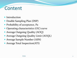
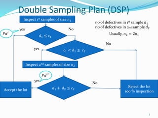
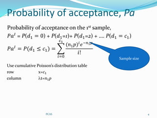
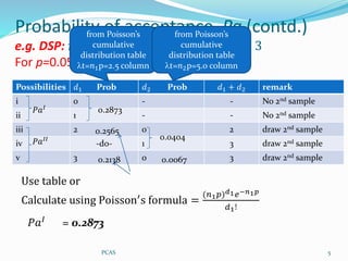
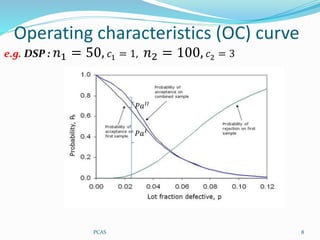
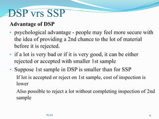
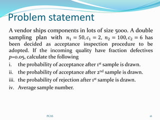
PCAS 1
Dr C K Biswas
Asso Prof.
Dept of ME
Content
 Introduction
 Double Sampling Plan (DSP)
 Probability of acceptance, Pa
 Operating characteristics (OC) curve
 Average Outgoing Quality (AOQ)
 Average Outgoing Quality Limit (AOQL)
 Average Sample Number (ASN)
 Average Total Inspection(ATI)
PCAS 2
Double Sampling Plan (DSP)
3
Inspect 1st samples of size 𝑛1
yes No
𝑑1 ≤ 𝑐1
Accept the lot
Reject the lot
100 % inspection
𝑃𝑎𝐼
no of defectives in 1st sample 𝑑1
no of defectives in 2nd sample 𝑑2
𝑐1 < 𝑑1 ≤ 𝑐2
Inspect 2nd samples of size 𝑛2
yes
No
𝑑1 + 𝑑2 ≤ 𝑐2
yes
No
𝑃𝑎𝐼𝐼
Usually, 𝑛2 = 2𝑛1
Probability of acceptance, Pa
PCAS 4
Probability of acceptance on the 1st sample,
𝑃𝑎𝐼 = P(𝑑1 = 0) + P(𝑑1=1)+ P(𝑑1=2) + …. P(𝑑1 = 𝑐1)
𝑃𝑎𝐼 = 𝑃(𝑑1 ≤ 𝑐1) =
𝑖=0
𝑐1
(𝑛1𝑝)𝑖
𝑒−𝑛1𝑝
𝑖!
Sample size
Use cumulative Poisson’s distribution table
row x=𝑐1
column t=𝑛1p
e.g. DSP: 𝑛1 = 50, 𝑐1 = 1, 𝑛2 = 100, 𝑐2 = 3
For p=0.05
PCAS 5
𝑃𝑎𝐼 = 0.2873
Probability of acceptance, Pa (contd.)
Possibilities 𝑑1 Prob 𝑑2 Prob 𝑑1 + 𝑑2 remark
i 0 - - No 2nd sample
ii 1 - - No 2nd sample
iii 2 0 2 draw 2nd sample
iv -do- 1 3 draw 2nd sample
v 3 0 3 draw 2nd sample
𝑃𝑎𝐼
𝑃𝑎𝐼𝐼
0.2873
0.0404
0.0067
from Poisson’s
cumulative
distribution table
t=𝑛1p=2.5 column
from Poisson’s
cumulative
distribution table
t=𝑛2p=5.0 column
0.2565
0.2138
Use table or
Calculate using Poisson′s formula =
(𝑛1𝑝)𝑑1𝑒−𝑛1𝑝
𝑑1!
Probability of acceptance, Pa (contd.)
Probability of acceptance after 2nd sample,
𝑃𝑎𝐼𝐼
= P(𝑐1 < 𝑑1 ≤ 𝑐2) P(𝑑1 + 𝑑2 ≤ 𝑐2)
PCAS 6
Prob of
drawing 2nd
sample
Prob of combined no
of defectives ≤ 𝑐2
𝑃𝑎𝐼𝐼
=
= 0.2565 x 0.0404 + 0.2138 x 0.0067
= 0.0118
+ P(𝑑1=3)P(𝑑2 = 0)
+ P(𝑑2 = 1)}
P(𝑑1 = 2) {P(𝑑2 = 0)
All numerical values are from the table in previous slide
Probability of acceptance, Pa (contd.)
PCAS 7
𝐏𝐚 = 𝑷𝒂𝑰 + 𝑷𝒂𝑰𝑰 = 𝟎. 𝟐𝟖𝟕𝟑 + 𝟎. 𝟎𝟏𝟐𝟎 = 𝟎. 𝟐𝟗𝟗𝟑
Pa is a function of p
Operating characteristics (OC) curve
PCAS 8
e.g. DSP : 𝑛1 = 50, 𝑐1 = 1, 𝑛2 = 100, 𝑐2 = 3
𝑃𝑎𝐼
𝑃𝑎𝐼𝐼
9
Inspect 1st samples of size 𝑛1
yes No
𝑑1 ≤ 𝑐1
Accept the lot
Reject the lot
100 % inspection
𝑃𝑎𝐼
𝑐1 < 𝑑1 ≤ 𝑐2
Inspect 2nd samples of size 𝑛2
yes
No
𝑑1 + 𝑑2 ≤ 𝑐2
yes
No
𝑃𝑎𝐼𝐼
Average Outgoing Quality (AOQ)
AOQ=
𝑃𝑎𝐼 𝑝𝑁−𝑝𝑛1 +𝑃𝑎𝐼𝐼(𝑝𝑁−𝑝𝑛1−𝑝𝑛2)
𝑁
𝑃𝑎𝐼(𝑝𝑁 − 𝑝𝑛1)
Incoming quality p
No of defectives in lot pN
𝑃𝑎𝐼𝐼
(𝑝𝑁 − 𝑝𝑛1 − 𝑝𝑛2)
Average Outgoing Quality Limit
PCAS 10
AOQL
11
Inspect 1st samples of size 𝑛1
yes No
𝑑1 ≤ 𝑐1
Accept the lot
Reject the lot
100 % inspection
𝑃𝑎𝐼
𝑐1 < 𝑑1 ≤ 𝑐2
Inspect 2nd samples of size 𝑛2
yes
No
𝑑1 + 𝑑2 ≤ 𝑐2
yes
No
𝑃𝑎𝐼𝐼
ATI=𝑃𝑎𝐼𝑛1 + 𝑃𝑎𝐼𝐼𝑛2 + (1 − 𝑃𝑎𝐼−𝑃𝑎𝐼𝐼)𝑁
𝑃𝑎𝐼
𝑛1
𝑃𝑎𝐼𝐼𝑛2
Average Total Inspection(ATI)
Incoming quality p
No of defectives in lot pN
(1 − 𝑃𝑎𝐼
−𝑃𝑎𝐼𝐼
)𝑁
12
Inspect 1st samples of size 𝑛1
yes No
𝑑1 ≤ 𝑐1
Accept the lot
Reject the lot
100 % inspection
𝑐1 < 𝑑1 ≤ 𝑐2
Inspect 2nd samples of size 𝑛2
yes
No
𝑑1 + 𝑑2 ≤ 𝑐2
yes
No
ASN=𝑃1𝑛1 + (𝑛1 + 𝑛2)(1 − 𝑃1) = 𝑛1 + 𝑛2(1 − 𝑃1)
Average Sample Number (ASN)
𝑃1 = P{lot is accepted on the 1st sample}
+ P{lot is rejected on the 1st sample}
PCAS 13
DSP vrs SSP
PCAS 14
Advantage of DSP
• psychological advantage - people may feel more secure with
the idea of providing a 2nd chance to the lot of material
before it is rejected.
• if a lot is very bad or if it is very good, it can be either
rejected or accepted with smaller 1st sample
• Suppose 1st sample in DSP is smaller than for SSP
If lot is accepted or reject on 1st sample, cost of inspection is
lower
Also possible to reject a lot without completing inspection of 2nd
sample
DSP vrs SSP (contd.)
PCAS 15
Disadvantage of DSP
• DSP needs more administrative effort than SSP
• If incoming lots quality, p close to the AQL and
consistent, the SSP is more economical than DSP
Problem statement
A vendor ships components in lots of size 5000. A double
sampling plan with 𝑛1 = 50, 𝑐1 = 2, 𝑛2 = 100, 𝑐2 = 6 has
been decided as acceptance inspection procedure to be
adopted. If the incoming quality have fraction defectives
p=0.05, calculate the following
i. the probability of acceptance after 1st sample is drawn.
ii. the probability of acceptance after 2nd sample is drawn.
iii. the probability of rejection after 1st sample is drawn.
iv. Average sample number.
PCAS 16
possibilities 𝑑1 Prob 𝑑2 Prob 𝑑1 + 𝑑2 remark
i 0 - - No 2nd sample
ii 1 - - No 2nd sample
iii 2 - - No 2nd sample
iv 3 0 3 draw 2nd sample
v -do- 1 4 draw 2nd sample
vi -do- 2 5 draw 2nd sample
vii -do- 3 6 draw 2nd sample
viii 4 0 4 draw 2nd sample
ix -do- 1 5 draw 2nd sample
x -do- 2 6 draw 2nd sample
xi 5 0 5 draw 2nd sample
xii -do- 1 6 draw 2nd sample
xiii 6 0 6 draw 2nd sample
PCAS 17
Solution
𝑃𝑎𝐼
𝑃𝑎𝐼𝐼
0.5438
from Poisson’s cumulative
distribution table t=𝑛1p=2.5
column
from Poisson’s cumulative
distribution table t=𝑛2p=5.0
column
0.2650
0.1247
0.0404
0.0067
0.2138
0.1336
0.0668
0.0278
Solution (contd.)
i. Probability of acceptance after 1st sample, 𝑃𝑎𝐼
= 0.5438
ii. 𝑃𝑎𝐼𝐼
= P(𝑑1 = 3){P(𝑑2 = 0) + P(𝑑2 = 1) + P(𝑑2 = 2) + P(𝑑2 = 3)}
+ P(𝑑1 = 4){P(𝑑2 = 0) + P(𝑑2 = 1) + P(𝑑2 = 2) }
+P(𝑑1 = 5){P(𝑑2 = 0) + P(𝑑2 = 1)}
+P(𝑑1 = 6){P(𝑑2 = 0) }
= 0.2138 x 0.2650 + 0.1336 x 0.1247 + 0.0668 x 0.0404 +
0.0278 x 0.0067
= 0.0762
PCAS 18
All numerical values are from the table in previous slide
Solution (contd.)
iii. Probability of rejecting after 1st sample,
𝑃𝑟𝐼
= P(𝑑1 ≥ 7) = 1- P(𝑑1 ≤ 6) = 1- 0.9858 = 0.0142
iv. ASN= 𝑛1 + 𝑛2(1 − 𝑃1)
Where 𝑃1 = 𝑃(𝑑1 ≤ 2) + P (𝑑1≥ 7)
= 0.5438 + 0.0142
= 0.558
So, ASN= 50 + 100 (1- 0.558) = 94.2
PCAS 19
PCAS 20

12 Acceptance sampling DSP.ppsx

  • 1.
    PCAS 1 Dr CK Biswas Asso Prof. Dept of ME
  • 2.
    Content  Introduction  DoubleSampling Plan (DSP)  Probability of acceptance, Pa  Operating characteristics (OC) curve  Average Outgoing Quality (AOQ)  Average Outgoing Quality Limit (AOQL)  Average Sample Number (ASN)  Average Total Inspection(ATI) PCAS 2
  • 3.
    Double Sampling Plan(DSP) 3 Inspect 1st samples of size 𝑛1 yes No 𝑑1 ≤ 𝑐1 Accept the lot Reject the lot 100 % inspection 𝑃𝑎𝐼 no of defectives in 1st sample 𝑑1 no of defectives in 2nd sample 𝑑2 𝑐1 < 𝑑1 ≤ 𝑐2 Inspect 2nd samples of size 𝑛2 yes No 𝑑1 + 𝑑2 ≤ 𝑐2 yes No 𝑃𝑎𝐼𝐼 Usually, 𝑛2 = 2𝑛1
  • 4.
    Probability of acceptance,Pa PCAS 4 Probability of acceptance on the 1st sample, 𝑃𝑎𝐼 = P(𝑑1 = 0) + P(𝑑1=1)+ P(𝑑1=2) + …. P(𝑑1 = 𝑐1) 𝑃𝑎𝐼 = 𝑃(𝑑1 ≤ 𝑐1) = 𝑖=0 𝑐1 (𝑛1𝑝)𝑖 𝑒−𝑛1𝑝 𝑖! Sample size Use cumulative Poisson’s distribution table row x=𝑐1 column t=𝑛1p
  • 5.
    e.g. DSP: 𝑛1= 50, 𝑐1 = 1, 𝑛2 = 100, 𝑐2 = 3 For p=0.05 PCAS 5 𝑃𝑎𝐼 = 0.2873 Probability of acceptance, Pa (contd.) Possibilities 𝑑1 Prob 𝑑2 Prob 𝑑1 + 𝑑2 remark i 0 - - No 2nd sample ii 1 - - No 2nd sample iii 2 0 2 draw 2nd sample iv -do- 1 3 draw 2nd sample v 3 0 3 draw 2nd sample 𝑃𝑎𝐼 𝑃𝑎𝐼𝐼 0.2873 0.0404 0.0067 from Poisson’s cumulative distribution table t=𝑛1p=2.5 column from Poisson’s cumulative distribution table t=𝑛2p=5.0 column 0.2565 0.2138 Use table or Calculate using Poisson′s formula = (𝑛1𝑝)𝑑1𝑒−𝑛1𝑝 𝑑1!
  • 6.
    Probability of acceptance,Pa (contd.) Probability of acceptance after 2nd sample, 𝑃𝑎𝐼𝐼 = P(𝑐1 < 𝑑1 ≤ 𝑐2) P(𝑑1 + 𝑑2 ≤ 𝑐2) PCAS 6 Prob of drawing 2nd sample Prob of combined no of defectives ≤ 𝑐2 𝑃𝑎𝐼𝐼 = = 0.2565 x 0.0404 + 0.2138 x 0.0067 = 0.0118 + P(𝑑1=3)P(𝑑2 = 0) + P(𝑑2 = 1)} P(𝑑1 = 2) {P(𝑑2 = 0) All numerical values are from the table in previous slide
  • 7.
    Probability of acceptance,Pa (contd.) PCAS 7 𝐏𝐚 = 𝑷𝒂𝑰 + 𝑷𝒂𝑰𝑰 = 𝟎. 𝟐𝟖𝟕𝟑 + 𝟎. 𝟎𝟏𝟐𝟎 = 𝟎. 𝟐𝟗𝟗𝟑 Pa is a function of p
  • 8.
    Operating characteristics (OC)curve PCAS 8 e.g. DSP : 𝑛1 = 50, 𝑐1 = 1, 𝑛2 = 100, 𝑐2 = 3 𝑃𝑎𝐼 𝑃𝑎𝐼𝐼
  • 9.
    9 Inspect 1st samplesof size 𝑛1 yes No 𝑑1 ≤ 𝑐1 Accept the lot Reject the lot 100 % inspection 𝑃𝑎𝐼 𝑐1 < 𝑑1 ≤ 𝑐2 Inspect 2nd samples of size 𝑛2 yes No 𝑑1 + 𝑑2 ≤ 𝑐2 yes No 𝑃𝑎𝐼𝐼 Average Outgoing Quality (AOQ) AOQ= 𝑃𝑎𝐼 𝑝𝑁−𝑝𝑛1 +𝑃𝑎𝐼𝐼(𝑝𝑁−𝑝𝑛1−𝑝𝑛2) 𝑁 𝑃𝑎𝐼(𝑝𝑁 − 𝑝𝑛1) Incoming quality p No of defectives in lot pN 𝑃𝑎𝐼𝐼 (𝑝𝑁 − 𝑝𝑛1 − 𝑝𝑛2)
  • 10.
    Average Outgoing QualityLimit PCAS 10 AOQL
  • 11.
    11 Inspect 1st samplesof size 𝑛1 yes No 𝑑1 ≤ 𝑐1 Accept the lot Reject the lot 100 % inspection 𝑃𝑎𝐼 𝑐1 < 𝑑1 ≤ 𝑐2 Inspect 2nd samples of size 𝑛2 yes No 𝑑1 + 𝑑2 ≤ 𝑐2 yes No 𝑃𝑎𝐼𝐼 ATI=𝑃𝑎𝐼𝑛1 + 𝑃𝑎𝐼𝐼𝑛2 + (1 − 𝑃𝑎𝐼−𝑃𝑎𝐼𝐼)𝑁 𝑃𝑎𝐼 𝑛1 𝑃𝑎𝐼𝐼𝑛2 Average Total Inspection(ATI) Incoming quality p No of defectives in lot pN (1 − 𝑃𝑎𝐼 −𝑃𝑎𝐼𝐼 )𝑁
  • 12.
    12 Inspect 1st samplesof size 𝑛1 yes No 𝑑1 ≤ 𝑐1 Accept the lot Reject the lot 100 % inspection 𝑐1 < 𝑑1 ≤ 𝑐2 Inspect 2nd samples of size 𝑛2 yes No 𝑑1 + 𝑑2 ≤ 𝑐2 yes No ASN=𝑃1𝑛1 + (𝑛1 + 𝑛2)(1 − 𝑃1) = 𝑛1 + 𝑛2(1 − 𝑃1) Average Sample Number (ASN) 𝑃1 = P{lot is accepted on the 1st sample} + P{lot is rejected on the 1st sample}
  • 13.
  • 14.
    DSP vrs SSP PCAS14 Advantage of DSP • psychological advantage - people may feel more secure with the idea of providing a 2nd chance to the lot of material before it is rejected. • if a lot is very bad or if it is very good, it can be either rejected or accepted with smaller 1st sample • Suppose 1st sample in DSP is smaller than for SSP If lot is accepted or reject on 1st sample, cost of inspection is lower Also possible to reject a lot without completing inspection of 2nd sample
  • 15.
    DSP vrs SSP(contd.) PCAS 15 Disadvantage of DSP • DSP needs more administrative effort than SSP • If incoming lots quality, p close to the AQL and consistent, the SSP is more economical than DSP
  • 16.
    Problem statement A vendorships components in lots of size 5000. A double sampling plan with 𝑛1 = 50, 𝑐1 = 2, 𝑛2 = 100, 𝑐2 = 6 has been decided as acceptance inspection procedure to be adopted. If the incoming quality have fraction defectives p=0.05, calculate the following i. the probability of acceptance after 1st sample is drawn. ii. the probability of acceptance after 2nd sample is drawn. iii. the probability of rejection after 1st sample is drawn. iv. Average sample number. PCAS 16
  • 17.
    possibilities 𝑑1 Prob𝑑2 Prob 𝑑1 + 𝑑2 remark i 0 - - No 2nd sample ii 1 - - No 2nd sample iii 2 - - No 2nd sample iv 3 0 3 draw 2nd sample v -do- 1 4 draw 2nd sample vi -do- 2 5 draw 2nd sample vii -do- 3 6 draw 2nd sample viii 4 0 4 draw 2nd sample ix -do- 1 5 draw 2nd sample x -do- 2 6 draw 2nd sample xi 5 0 5 draw 2nd sample xii -do- 1 6 draw 2nd sample xiii 6 0 6 draw 2nd sample PCAS 17 Solution 𝑃𝑎𝐼 𝑃𝑎𝐼𝐼 0.5438 from Poisson’s cumulative distribution table t=𝑛1p=2.5 column from Poisson’s cumulative distribution table t=𝑛2p=5.0 column 0.2650 0.1247 0.0404 0.0067 0.2138 0.1336 0.0668 0.0278
  • 18.
    Solution (contd.) i. Probabilityof acceptance after 1st sample, 𝑃𝑎𝐼 = 0.5438 ii. 𝑃𝑎𝐼𝐼 = P(𝑑1 = 3){P(𝑑2 = 0) + P(𝑑2 = 1) + P(𝑑2 = 2) + P(𝑑2 = 3)} + P(𝑑1 = 4){P(𝑑2 = 0) + P(𝑑2 = 1) + P(𝑑2 = 2) } +P(𝑑1 = 5){P(𝑑2 = 0) + P(𝑑2 = 1)} +P(𝑑1 = 6){P(𝑑2 = 0) } = 0.2138 x 0.2650 + 0.1336 x 0.1247 + 0.0668 x 0.0404 + 0.0278 x 0.0067 = 0.0762 PCAS 18 All numerical values are from the table in previous slide
  • 19.
    Solution (contd.) iii. Probabilityof rejecting after 1st sample, 𝑃𝑟𝐼 = P(𝑑1 ≥ 7) = 1- P(𝑑1 ≤ 6) = 1- 0.9858 = 0.0142 iv. ASN= 𝑛1 + 𝑛2(1 − 𝑃1) Where 𝑃1 = 𝑃(𝑑1 ≤ 2) + P (𝑑1≥ 7) = 0.5438 + 0.0142 = 0.558 So, ASN= 50 + 100 (1- 0.558) = 94.2 PCAS 19
  • 20.