113657800 ofdm-simulation-in-matlab

OFDM SIMULATION in MATLAB
A Senior Project
Presented to the Faculty of
California Polytechnic State University
San Luis Obispo
In Partial Fulfillment
of the Requirements for the Degree of
Bachelor of Science in Electrical Engineering
By
Paul Guanming Lin
June 2010

ii
Table of Contents
List of Figures and Tables ................................................................................................................. iii
Chapter 1 – INTRODUCTION.............................................................................................................. 1
Chapter 2 – BACKGROUND................................................................................................................ 3
2.1 – OFDM Basics............................................................................................................................... 3
2.2 – Overview of This OFDM Simulation Project............................................................................... 6
Chapter 3 – DESIGN and IMPLEMENTATION...................................................................................... 8
3.1 – Overview .................................................................................................................................... 8
3.2 – System Configurations and Parameters................................................................................... 10
3.3 – Input and Output...................................................................................................................... 11
3.4 – OFDM Transmitter ................................................................................................................... 13
3.4.1 – Frame Guards ................................................................................................................... 13
3.4.2 – OFDM Modulator.............................................................................................................. 14
3.5 – Communication Channel.......................................................................................................... 17
3.6 – OFDM Receiver ........................................................................................................................ 18
3.6.1 – Frame detector ................................................................................................................. 18
3.6.2 – Demodulation Status Indicator......................................................................................... 18
3.6.3 – OFDM Demodulator.......................................................................................................... 19
3.7 – Error Calculations..................................................................................................................... 21
3.8 – Plotting..................................................................................................................................... 23
Chapter 4 – TEST RESULTS............................................................................................................... 25
Chapter 5 – CONCLUSION................................................................................................................ 34
Bibliography.................................................................................................................................... 35
Appendix A – Glossary and Acronyms............................................................................................. 36
Appendix B – A Trial of this OFDM MATLAB Simulation .................................................................. 37
B.1 – Screen Log................................................................................................................................ 37
B.2 – Input and Output Images......................................................................................................... 38
B.3 – Transmitter Plots...................................................................................................................... 39
B.4 – Receiver Plots........................................................................................................................... 40
Appendix C – Complete Source Codes for this Project..................................................................... 41
C.1 – Main Program File (OFDM_SIM.m).......................................................................................... 41
C.2 – System Configuration Script File (ofdm_parameters.m) ......................................................... 47
C.3 – Data Word/Symbol Size Conversion Function File (ofdm_base_convert.m)........................... 49
C.4 – Modulation Function File (ofdm_modulate.m) ....................................................................... 50
C.5 – Frame Detection Function File (ofdm_frame_detect.m)......................................................... 53
C.6 – Demodulation Function File (ofdm_demod.m) ....................................................................... 54

iii
List of Figures and Tables
List of Figures
Figure 1 – Cyclic Extension Tolerance ..................................................................................................... 1
Figure 2 – Effectiveness of the Cyclic Extension...................................................................................... 1
Figure 3 – Block Diagram of an OFDM System........................................................................................ 1
Figure 4 – OFDM carriers allocated to IFFT bins...................................................................................... 1
Figure 5 – Modulated Signal (single frame)............................................................................................. 1
Figure 6 – Modulated Signal (multiple frames)....................................................................................... 1
Figure 7 – data_tx_matrix ....................................................................................................................... 1
Figure 8 – Differentiated matrix.............................................................................................................. 1
Figure 9 – pre-IFFT matrix ....................................................................................................................... 1
Figure 10 – Modulated Matrix................................................................................................................. 1
Figure 11 – Time Guard Removal ............................................................................................................ 1
Figure 12 – Received Data Extracted from FFT bins................................................................................ 1
Figure 13 – Differential Demodulation.................................................................................................... 1
Figure 14 – Program Runtime ................................................................................................................. 1
Figure 15 – BER vs M-PSK........................................................................................................................ 1
Figure 16 – BER vs SNR............................................................................................................................ 1
Figure 17 – Pixel Error vs SNR.................................................................................................................. 1
Figure 18 – Original Image....................................................................................................................... 1
Figure 19 - Received Images using BPSK ................................................................................................. 1
Figure 20 – Received Images using QPSK ................................................................................................ 1
Figure 21 – Received Images using 16-PSK.............................................................................................. 1
Figure 22 – Received Images using 256-PSK............................................................................................ 1
Figure 23 – OFDM Received Image ......................................................................................................... 1
Figure 24 – Original Image....................................................................................................................... 1
Figure 25 – OFDM Transmitter Plots....................................................................................................... 1
Figure 26 – OFDM Receiver Plots............................................................................................................ 1
List of Tables
Table 1 – User Input Validity Protection ................................................................................................. 1
Table 2 – OFDM Transmission Summary................................................................................................. 1
Table 3 – Error Calculations..................................................................................................................... 1
Table 4 – Parameters of Simulation in Appendix B ............................................................................... 25
Table 5 – Parameters for BER/SNR Analysis............................................................................................ 1
Table 6 – OFDM Simulation Log .............................................................................................................. 1

1
Chapter 1 – INTRODUCTION
In a single carrier communication system, the symbol period must be much
greater than the delay time in order to avoid inter-symbol interference (ISI) [1]. Since
data rate is inversely proportional to symbol period, having long symbol periods
means low data rate and communication inefficiency. A multicarrier system, such as
FDM (aka: Frequency Division Multiplexing), divides the total available bandwidth
in the spectrum into sub-bands for multiple carriers to transmit in parallel [2]. An
overall high data rate can be achieved by placing carriers closely in the spectrum.
However, inter-carrier interference (ICI) will occur due to lack of spacing to separate
the carriers. To avoid inter-carrier interference, guard bands will need to be placed in
between any adjacent carriers, which results in lowered data rate.
OFDM (aka: Orthogonal Frequency Division Multiplexing) is a multicarrier
digital communication scheme to solve both issues. It combines a large number of
low data rate carriers to construct a composite high data rate communication system.
Orthogonality gives the carriers a valid reason to be closely spaced, even overlapped,
without inter-carrier interference. Low data rate of each carrier implies long symbol
periods, which greatly diminishes inter-symbol interference [3].
Although the idea of OFDM started back in 1966 [4], it has never been widely
utilized until the last decade when it “becomes the modem of choice in wireless
applications” [5]. It is now interested enough to experiment some insides of OFDM.

2
The objective of this project is to demonstrate the concept and feasibility of an
OFDM system, and investigate how its performance is changed by varying some of
its major parameters. This objective is met by developing a MATLAB program to
simulate a basic OFDM system. From the process of this development, the
mechanism of an OFDM system can be studied; and with a completed MATLAB
program, the characteristics of an OFDM system can be explored.

3
Chapter 2 – BACKGROUND
2.1 – OFDM Basics
In digital communications, information is expressed in the form of bits. The
term symbol refers to a collection, in various sizes, of bits [6]. OFDM data are
generated by taking symbols in the spectral space using M-PSK, QAM, etc, and
convert the spectra to time domain by taking the Inverse Discrete Fourier Transform
(IDFT). Since Inverse Fast Fourier Transform (IFFT) is more cost effective to
implement, it is usually used instead [3]. Once the OFDM data are modulated to time
signal, all carriers transmit in parallel to fully occupy the available frequency
bandwidth [7]. During modulation, OFDM symbols are typically divided into frames,
so that the data will be modulated frame by frame in order for the received signal be
in sync with the receiver. Long symbol periods diminish the probability of having
inter-symbol interference, but could not eliminate it. To make ISI nearly eliminated,
a cyclic extension (or cyclic prefix)
is added to each symbol period. An
exact copy of a fraction of the
cycle, typically 25% of the cycle,
taken from the end is added to the
front. This allows the demodulator
to capture the symbol period with
Figure 1 – Cyclic Extension Tolerance

4
an uncertainty of up to the length of a cyclic extension and still obtain the correct
information for the entire symbol period. As shown in Figure 1 [8], a guard period,
another name for the cyclic extension, is the amount of uncertainty allowed for the
receiver to capture the starting point of a symbol period, such that the result of FFT
still has the correct information. In Figure 2 [9], a comparison between a precisely
detected symbol period and a delayed detection illustrates the effectiveness of the
cyclic extension.
OFDM Parameters and Characteristics
The number of carriers in an OFDM system is not only limited by the
available spectral bandwidth, but also by the IFFT size (the relationship is described
by:
_
number of carriers 2
2
ifft size
≤ − ), which is determined by the complexity of the
system [10]. The more complex (also more costly) the OFDM system is, the higher
IFFT size it has; thus a higher number of carriers can be used, and higher data
Figure 2 – Effectiveness of the Cyclic Extension

5
transmission rate achieved. The choice of M-PSK modulation varies the data rate and
Bit Error Rate (BER). The higher order of PSK leads to larger symbol size, thus less
number of symbols needed to be transmitted, and higher data rate is achieved. But
this results in a higher BER since the range of 0-360 degrees of phases will be divided
into more sub-regions, and the smaller size of sub-regions is required, thereby
received phases have higher chances to be decoded incorrectly. OFDM signals have
high peak-to-average ratio, therefore it has a relatively high tolerance of peak power
clipping due to transmission limitations.
Orthogonality
The key to OFDM is maintaining orthogonality of the carriers. If the integral
of the product of two signals is zero over a time period, then these two signals are
said to be orthogonal to each other. Two sinusoids with frequencies that are integer
multiples of a common frequency can satisfy this criterion. Therefore, orthogonality
is defined by:
where n and m are two unequal integers; fo is the fundamental frequency; T is the
period over which the integration is taken. For OFDM, T is one symbol period and fo
set to to
1
T
for optimal effectiveness [11 and 12].
0
cos(2 )cos(2 ) 0 ( )
T
o onf t mf t dt n mπ π = ≠∫

6
2.2 – Overview of This OFDM Simulation Project
Since MATLAB has a built-in function “ifft()” which performs Inverse Fast
Fourier Transform, IFFT is opted for the development of this simulation. Six m-files
are written to develop this MATLAB program of OFDM simulation. One of them is
the main program script file, which is the only file that needs to be run, while other
m-files will be invoked accordingly. A 256-grayscale bitmap image is required as the
source input. Another bitmap image file will be generated at the end of the
simulation as the output. Three MATLAB data storage files (err_calc.mat,
ofdm_parameters.mat, and received.mat) are generated during the simulation.
err_calc.mat is to archive the baseband data before the transmission, and be retrieved
at the end of the simulation for the purpose of error calculations.
ofdm_parameters.mat is to archive the parameters initialized at the beginning of the
simulation and reserve them for the receiver to use later. In the reality, the receiver
would always have these parameters; in this simulation, these parameters are
configured by the user at the beginning, so they are passed to the receiver by
ofdm_parameters.mat as if being preset in the receiver. received.mat stores the time
signal after it travels through the channel, and lets the receiver to read it directly.
When the simulation proceeds through the OFDM transmitter and communication
channel, it pauses and waits for the user to trigger for proceeding to the receiver. The
reason for using the last two *mat files is that as soon as the OFDM receiver
proceeds, the program will clear all data/variables stored in MATLAB workspace.
This is to simulate the real situation in which OFDM receivers have no knowledge of

7
the data except for the received signal at the exit of the communication channel.
Simulation runtime for both the transmitter and receiver are measured and shown on
MATLAB command screen as a rough measurement of relative data rate.
Appendix B shows full information of a trial of the OFDM simulation while
Appendix C contains all the MATLAB source codes for this project with detailed
comments for explanations.

8
Chapter 3 – DESIGN and IMPLEMENTATION
3.1 – Overview
Figure 3 shows a block diagram of a generic OFDM system. ADC, DAC, and
RF front-ends (Amplification, RF upconversion/downconversion, etc.) are not
simulated in this project. This MATLAB simulation program consists of six files.
OFDM_SIM.m shall be run while other m-files will be invoked accordingly.
Source data for this simulation is taken from an 8-bit grayscale (256 gray
levels) bitmap image file (*.bmp) based on the user’s choice. The image data will
then be converted to the symbol size (bits/symbol) determined by the choice of M-
PSK from four variations provided by this simulation. The converted data will then
be separated into multiple frames by the OFDM transmitter. The OFDM modulator
modulates the data frame by frame. Before the exit of the transmitter, the modulated
frames of time signal are cascaded together along with frame guards inserted in
between as well as a pair of identical headers added to the beginning and end of the
data stream. The communication channel is modeled by adding Gaussian white noise
and amplitude clipping effect.
The receiver detects the start and end of each frame in the received signal by
an envelope detector. Each detected frame of time signal is then demodulated into
useful data. The modulated data is then converted back to 8-bit word size data used
for generating an output image file of the simulation.
Error calculations are performed at the end of the program. Representative
plots are shown throughout the execution of this simulation.

9
OFDM Transmitter
OFDM Demodulator
source
data
from
input
bmp
file
serial
to
parallel
IFFT bins
allocation
DPSK
modulation
(1, 2, 4,
or 8 bits)
IFFT
cyclic
extension
addition
parallel
to
serial
frames
divider
cascade
frames;
add frame
guards,
header
and trailer
RF
front-end
communication
channel
RF
front-end
frames
detection
DAC
ADC
received
data to
generate
output
bmp file
extract
carriers
from
FFT bins
FFT
cyclic
extension
removal
serial
to
parallel
parallel
to
serial
DPSK
demodulation
(1, 2, 4,
or 8 bits)
cascade
frames
OFDM Demodulator
OFDM Receiver
Figure3–BlockDiagramofanOFDMSystem

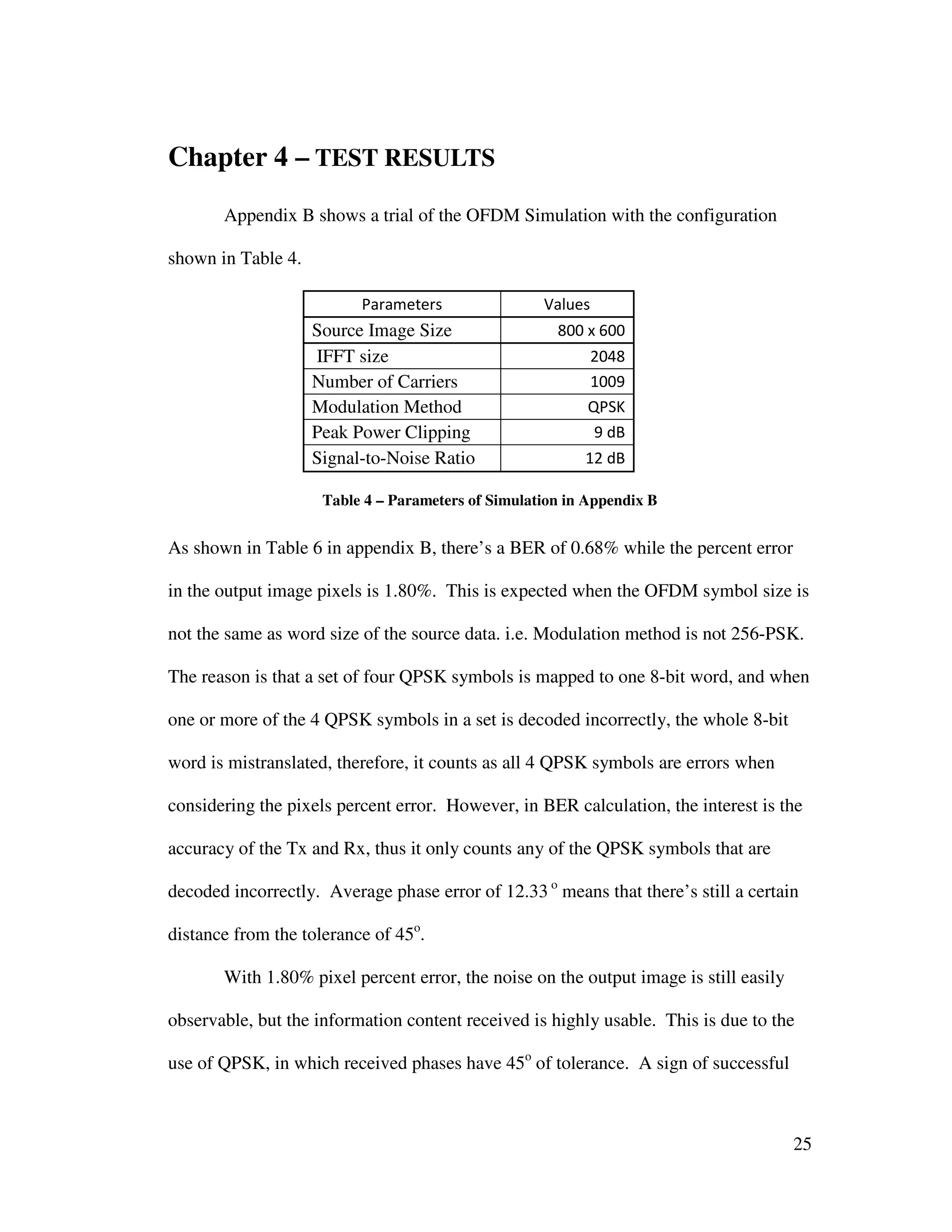
10
3.2 – System Configurations and Parameters
At the beginning of this simulation MATLAB program, a script file
ofdm_parameters.m is invoked, which initializes all required OFDM parameters and
program variables to start the simulation. Some variables are entered by the user.
The rest are either fixed or derived from the user-input and fixed variables. The user-
input variables include:
1) Input file – an 8-bit grayscale (256 gray levels) bitmap file (*.bmp);
2) IFFT size – an integer of a power of two;
3) Number of carriers – not greater than [(IFFT size)/2 – 2];
4) Digital modulation method – BPSK, QPSK, 16-PSK, or 256-PSK;
5) Signal peak power clipping in dB;
6) Signal-to-Noise Ratio in dB.
The number of carriers needs to be no more than [(IFFT size)/2 – 2], because there
are as many conjugate carriers as the carriers, and one IFFT bin is reserved for DC
signal while
another IFFT bin
is for the
symmetrical point
at the Nyquist
frequency to
separate carriers
and conjugate carriers. All user-inputs are checked for validity and the program will
##########################################
#*********** OFDM Simulation ************#
##########################################
source data filename: abc
"abc" does not exist in current directory.
source data filename: cat.bmp
Output file will be: cat_OFDM.bmp
IFFT size: 1200
IFFT size must be at least 8 and power of 2.
IFFT size: 1024
Number of carriers: 1000
Must NOT be greater than ("IFFT size"/2-2)
Modulation(1=BPSK, 2=QPSK, 4=16PSK, 8=256PSK): 3
Only 1, 2, 4, or 8 can be choosen
Amplitude clipping introduced by communication channel (in dB): 6
Signal-to-Noise Ratio (SNR) in dB: 10
Table 1 – User Input Validity Protection

11
request the user to correct any incorrect fields with brief guidelines provided. An
example is shown in Table 1. This script also determines how the carriers and
conjugate carriers are
allocated into the
IFFT bins, based on
the IFFT size and
number of carriers
defined by the user.
Figure 4 shows an
example of 120
carriers and 120
conjugate carriers
spreading out on 256
IFFT bins. Refer to appendix C.2 for more details.
3.3 – Input and Output
The program reads data from an input image file and obtains an h-by-w matrix
where h is the height of the image and w is the width (in pixels). This matrix is
rearranged into a serial data stream. Since the input image is an 8-bit grayscale
bitmap, its word size is always 8 bits/word. The source data will then be converted to
the symbol size corresponding to the order of PSK chosen by the user.
ofdm_base_convert.m performs this conversion. It converts the original 8-bits/word
Figure 4 – OFDM carriers allocated to IFFT bins

12
data stream to a binary matrix with each column representing a symbol in the symbol
size of the selected PSK order. This binary matrix will then be converted to the data
stream with such a symbol size, which is the baseband to enter the OFDM transmitter.
For example, when QPSK (4 bits/word) is selected, a data stream in 8-bits/word is
[36, 182, 7] will go through the following process:
36 7 182
[36, 7, 182] [2, 4, 0, 7, 11, 6]
three 8-bit words binary matrix six4-bit symbols
At the exit of the OFDM receiver, a demodulated data stream needs to go
through the base conversion again to return to 8-bits/word. This time, since the PSK
symbol size might be less than 8 bits/symbol, ofdm_base_convert.m would trim the
data stream to a multiple of 8/symbol-size before the base conversion in order to let
each symbol conversion have sufficient bits. If the OFDM receiver does not detect
all the data frames at the exactly correct locations, demodulated data may not be in
the same length as the transmitted data stream. [2, 4, 0, 7, 11] may be the received
data stream instead of [2, 4, 0, 7, 11, 6]. For this instance, “11” is dropped and only
[2, 4, 0, 7] will be converted for generating the output image.
The output image:
Sometimes the OFDM receiver’s outcome may also happen to be a data
stream that is longer than the original transmitted data stream due to some
imprecision processing caused by channel noise. In such cases, the received data
0 0 0 0 1 0
0 1 0 1 0 1
1 0 0 1 1 1
0 0 0 1 1 0
 
 
 
 
 
 

13
stream is trimmed to the length of the original data stream in order to fit the
dimensions of the original image.
On the contrary, the received data would more likely have a length less than
the original. In these cases, the program would consider the number of the full
missing rows as the amount to trim h, the height of the original image. Some
treatment is processed for the partially missing row if it exists. When one or more
full missing rows occur, the program shows a warning message informing the user
that the output image is in a smaller size than the original image. For the partially
missing row of received pixel data, the program would fill a number of pixels to make
it in the same length as all other rows. Each of these padded pixels would have the
same grayscale level as the pixel right above it in the image (one less row, same
column). This would make the partial missing row of pixels nearly seamless.
3.4 – OFDM Transmitter
3.4.1 – Frame Guards
The core of the OFDM transmitter is the modulator, which modulates the
input data stream frame by frame. Data is divided into frames based on the variable
symb_per_frame, which refers to the number of symbols per frame per carrier. It is
defined by: symb_per_frame = ceil(2^13/carrier_count). This limits the total
number of symbols per frame (symb_per_frame * carrier_count) within the
interval of [2^13, 2*(2^13-1)], or [8192, 16382]. However, the number of carriers
typically would not be much greater than 1000 in this simulation, thus the total

14
number of symbols per frame would typically be under 10,000. This is an
experimentally reasonable number of symbols that one frame should keep under for
this MATLAB program to run efficiently; thereby symb_per_frame is defined by the
equation shown above. If the total number of symbols in a data stream to be
transmitted is less than the total number of symbols per frame, the data would not be
divided into frames and would be modulated all at once. As shown in Figure 5, even
if the data stream is not
sufficiently long to be divided
into multiple frames, two frame
guards with all zero values and in a length of one symbol period are still added to
both ends of the modulated time signal. This is to assist the receiver to locate the
beginning of the substantial portion of the time signal. As shown in Figure 6, for
modulated signals with multiple frames, a frame guard is inserted in between any two
adjacent frames as well as both ends of the cascaded time signal. Finally, a pair of
headers is padded to both ends of the guarded series of frames. The headers are
scaled to the RMS level of the modulated time signal.
3.4.2 – OFDM Modulator
It is normal that the total number of transmitting data is not a multiple of the
number of carriers. To convert the input data stream from serial to parallel, the
Header
Frame
Guard
Header
Frame
Guard
Modulated
Signal
Figure 5 – Modulated Signal (single frame)
Figure 6 – Modulated Signal (multiple frames)
Frame
Guard
Modulated
Signal
Header
Frame
Guard
Header
Frame
Guard
Modulated
Signal

15
modulator must pad a number of zeros to the end of the data stream in order for the
data stream to fit into a 2-D matrix. Suppose a frame of data with 11,530 symbols is
being transmitted by 400 carriers with a capacity of 30
symbols/carrier. 470 zeros are padded at the end in order
for the data stream to form a 30-by-400 matrix, as shown
in Figure 7. Each column in the 2-D matrix represents a
carrier while each row represents one symbol period over all carriers.
Differential Phase Shift Keying (DPSK) Modulation
Before differential encoding can be operated on
each carrier (column of the matrix), an extra row of
reference data must be added on top of the matrix. The
modulator creates a row of uniformly random numbers
within an interval defined by the symbol size (order of PSK chosen) and patches it on
the top of the matrix. Figure 8 shows a 31-by-400 resulted matrix. For each column,
starting from the second row (the first actual data symbol), the value is changed to the
remainder of the sum of its previous row and itself over the symbol size (power 2 of
the PSK order). An illustration below shows how this operation is carried out for a
QPSK (symbol size = 22
= 4).
0
3
2
1
 
 
 
 
 
 
with [2] added as the reference becomes
2
0
3
2
1
 
 
 
 
 
 
  
, which is then differentiated to
2
2
1
3
0
 
 
 
 
 
 
  
Figure 7 – data_tx_matrix
400
DATA30
400
DATA
Reference Row
31
Figure 8 – Differentiated matrix

16
Every symbol in the differentiated matrix is translated to its corresponding phase
value from 0 to 360 degrees. Therefore,
2
2
1
3
0
 
 
 
 
 
 
  
is translated to
180
180
90
270
0
Ο
Ο
Ο
Ο
Ο
 
 
 
 
 
 
 
  
The modulator generates a DPSK matrix filled with complex numbers whose phases
are those translated phases and magnitudes are all ones. These complex numbers are
then converted to rectangular form for further processing.
IFFT: Spectral Space to Time Signal
Figure 9 shows that the matrix is widened to
IFFT size (for example: IFFT size = 1024) and becomes
a 31-by-1024 IFFT matrix. Since each column of the
DPSK matrix represents a carrier, their values are stored to the columns of the IFFT
matrix at the locations where their corresponding carriers should reside. Their
conjugate values are stored to the columns corresponding to the locations of the
conjugate carriers (refer to Figure 4). All other columns in the IFFT matrix are set to
zero. To obtain the transmitting time signal matrix, Inverse Fast Fourier Transform
(IFFT) of this matrix is taken. Only the real part of the IFFT result is useful, so the
imaginary part is discarded.
400
31
1024
DATA
Conjugate
DATA
400
Figure 9 – pre-IFFT matrix

17
Periodic Time Guard Insertion
An exact copy of the last 25% portion of each
symbol period (row of the matrix) is inserted to the
beginning. As shown in Figure 10, the matrix is
further widened to a width of 1280. This is the periodic time guard that helps the
receiver to synchronize when demodulating each symbol period of the received
signal. The matrix now becomes a modulated matrix. By converting it to a serial
form, a modulated time signal for one frame of data is generated.
3.5 – Communication Channel
Two properties of a typical communication channel are modeled. A variable
clipping in this MATLAB program is set by the user. Peak power clipping is
basically setting any data points with values over clipping below peak power to
clipping below peak power. The peak-to- RMS ratios of the transmitted signal
before and after the channel are shown for a comparison regarding this peak power
clipping effect. An example is shown in Table 2.
Channel noise is modeled by adding a white Gaussian noise (AWGN) defined
by:
31
1280
Figure 10 – Modulated Matrix
variance of the modulated signal
of AWGN =
linear SNR
σ
Summary of the OFDM transmission and channel modeling:
Peak to RMS power ratio at entrance of channel is: 14.893027 dB
Peak to RMS power ratio at exit of channel is: 11.502826 dB
#******** OFDM data transmitted in 5.277037 seconds ********#
Table 2 – OFDM Transmission Summary

18
It has a mean of zero and a standard deviation equaling the square root of the quotient
of the variance of the signal over the linear Signal-to-Noise Ratio, the dB value of
which is set by the user as well.
3.6 – OFDM Receiver
3.6.1 – Frame detector
A trunk of received signal in a selective length is processed by the frame
detector (ofdm_frame_detect.m) in order to determine the start of the signal frame.
For only the first frame, this selected portion is relatively larger for taking the header
into account. The selected portion of received signal is sampled to a shorter discrete
signal with a sampling rate defined by the system. A moving sum is taken over this
sampled signal. The index of the minimum of the sampled signal is approximately
the start of the frame guard while one symbol period further from this index is the
approximate location for the start of the useful signal frame. The frame detector will
then collect a moving sum of the input signal from about 10% of one symbol period
earlier than the approximate start of the frame guard to about one third of s symbol
period further than the approximate start of the useful signal frame. The first portion,
with a length of one less than a symbol period of this moving sum is discarded. The
first minimum of this moving sum is the detected start of the useful signal frame.
3.6.2 – Demodulation Status Indicator
As mentioned, received OFDM signal is typically demodulated frame by
frame. The OFDM receiver shows the progress of frames being demodulated.

19
However, the total number of frames may vary by a wide range depending on the
total amount of information transmitted via the OFDM system. It is a neat idea to
keep the number of displays for this progress within a reasonable range, so that the
MATLAB command screen is not overwhelmed by these status messages, nor the
amount of messages shown is less than useful. To achieve this, the first and last
frames are designed to show for sure, the rest would have to meet a condition:
rem(k,max(floor(num_frame/10),1))==0
where k is the variable to indicate the k-th frame being modulated, and num_frame
is the total number of frames. It means that for a total number of frames being 20 or
more, it only displays the n-th frame when n is an integer multiple of the round-down
integer of a tenth of the total number of frames; and for a total number of frames
being 19 or less, it shows every frame that is being modulated. This would keep the
total number of displays within the range from 11 to 19, provided that the total
number of frames is more than 10; otherwise, it simply shows as many messages as
the total number of frames.
3.6.3 – OFDM Demodulator
Like any typical modulation/demodulation, OFDM demodulation is basically
a reverse process of OFDM modulation. And like its modulator, the OFDM
demodulator demodulates the received data frame by frame unless the transmitted
data has length less than the designed total number of symbols per frame.

20
Periodic Time Guard Removal
The previous example used in section 3.4.2 “OFDM Modulator” shall
continue to be used for illustration. Figure 11 shows that after converting a frame of
discrete time signal from serial to parallel, a length of 25% of a symbol period is
discarded from all rows. Thus the remaining is then a number of discrete signals with
the length of one symbol period lined up in parallel.
FFT: Time Signal to Spectral Space
Fast Fourier Transform (FFT) of the received time signal is taken. This
results the spectrum of the received signal. As shown in Figure 12, the columns in
the locations of carriers are extracted to retrieve the complex matrix of the received
data.
Differential Phase Shift Keying (DPSK) Demodulation
The phase of every element in the complex matrix is converted into 0-360
degrees range and translated to one of the values within the symbol size. The
Figure 11 – Time Guard Removal
31
1280
31
1024
1024
31
400 400
DATA
Conjugate
DATA
400
DATA
Reference Row
31
Figure 12 – Received Data Extracted from FFT bins

21
translated values form a new matrix. The differential operation is performed in
parallel on this new matrix to retrieve the demodulated data. This differential
operation is basically calculating the difference between every two consecutive
symbols in a column of the matrix. As shown in Figure 13, the reference row is
removed during this operation. Finally, a parallel to serial operation is performed and
the demodulated data stream for this frame is obtained. Note that a series of zeros
may have been padded to the original data before transmission in order to make each
carrier have the same number of data symbols. Therefore, the modulator may have to
remove the padded zeros from the last portion of the demodulated data stream before
the final version of the received data can be obtained. The number of padded zeros is
calculated by taking the remainder of total number of data symbols over the number
of carriers.
3.7 – Error Calculations
Data loss
As mentioned in section 3.3 “Input and Output,” one or more of full rows of
pixels may be missing at the output of the receiver. In such cases, this program
400
DATA
Reference Row
31
400
DATA30
Figure 13 – Differential Demodulation

22
would show the number of missing data and the total number of data transmitted, as
well as the percentage of data loss, which is the quotient of the two.
Bit Error Rate (BER)
Demodulated data is compared to the original baseband data to find the total
number of errors. Dividing the total number of errors by total number of
demodulated symbols, the bit-error-rate (BER) is found.
Phase Error
During the OFDM demodulation, before being translated into symbol values
the received phase matrix is archived for calculating the average phase error, which is
defined by the difference between the received phase and the translated phase for the
corresponding symbol before transmission.
Percent Error of Pixels in the Received Image
All aforementioned error calculations are based on the OFDM symbols. What
is more meaningful for the end-user of the OFDM communication system is the
actual percent error of pixels in the received image. This is done by comparing the
received image and original image pixel by pixel.
Program Display
A summary showing the above error calculations is displayed at the end of the
program. In an example shown in Table 3, an 800-by-600 image is transmitted by
#**************** Summary of Errors ****************#
Data loss in this communication = 0.125000% (1200 out of 960000)
Total number of errors = 1174 (out of 958800)
Bit Error Rate (BER) = 0.122445%
Average Phase Error = 1.877366 (degree)
Percent error of pixels of the received image = 0.257708%
Table 3 – Error Calculations

23
400 carriers using an IFFT size of 1024, through a channel with 5 dB peak power
clipping and 30 dB SNR white Gaussian noise.
3.8 – Plotting
Seven graphs are plotted during this OFDM simulation:
1. Magnitudes of OFDM carrier data on IFFT bins;
Since all magnitudes are ONE, what this plot really shows is how the
carriers are spread out in the IFFT bins.
2. Phases translated from the OFDM data;
In this graph, it’s easy to see that the original data has a number of
possible levels equal to 2 raised to the power of symbol size.
3. Modulated time signal for one symbol period on one carrier;
4. Modulated time signal for one symbol period on multiple (limiting to six)
carriers;
5. Magnitudes of the received OFDM spectrum;
This is to be compared to the first graph.
6. Phases of the received OFDM spectrum;
This is to be compared to the second graph.
7. Polar plot of the received phases;
A successful OFDM transmission and reception should have this plot
show the grouping of the received phases clearly into 2^symbol-size
constellations.

24
The first four plots are derived from OFDM modulation while the last three are from
demodulation. None of these plots include a complete OFDM data packet. The first
three plots represent only the first symbol period in the first frame of data, whereas
the fourth plot represents up to the first six symbol periods in the first frame. Since
the first and last portion of the received/modulated data have higher probability of
getting errors due to imprecision in synchronization, a sample of symbol period used
by the fifth, sixth, and seventh plots is from the approximate middle of a frame, which
is also approximately the middle one among all data frames. However, it’s still
possible that the sample taken for the demodulation plots is still erroneous on certain
trials of this MATLAB simulation. It is important to note that even if the fifth, sixth,
and seventh plots don’t show reasonable information, the overall OFDM transmission
and reception would still likely be valid since these plots only represent one symbol
period among many. Appendix B provides a example of each of these seven plots.

25
Chapter 4 – TEST RESULTS
Appendix B shows a trial of the OFDM Simulation with the configuration
shown in Table 4.
Parameters Values
Source Image Size 800 x 600
IFFT size 2048
Number of Carriers 1009
Modulation Method QPSK
Peak Power Clipping 9 dB
Signal-to-Noise Ratio 12 dB
Table 4 – Parameters of Simulation in Appendix B
As shown in Table 6 in appendix B, there’s a BER of 0.68% while the percent error
in the output image pixels is 1.80%. This is expected when the OFDM symbol size is
not the same as word size of the source data. i.e. Modulation method is not 256-PSK.
The reason is that a set of four QPSK symbols is mapped to one 8-bit word, and when
one or more of the 4 QPSK symbols in a set is decoded incorrectly, the whole 8-bit
word is mistranslated, therefore, it counts as all 4 QPSK symbols are errors when
considering the pixels percent error. However, in BER calculation, the interest is the
accuracy of the Tx and Rx, thus it only counts any of the QPSK symbols that are
decoded incorrectly. Average phase error of 12.33 o
means that there’s still a certain
distance from the tolerance of 45o
.
With 1.80% pixel percent error, the noise on the output image is still easily
observable, but the information content received is highly usable. This is due to the
use of QPSK, in which received phases have 45o
of tolerance. A sign of successful

26
QPSK is shown in the third graph in Figure 26 with obvious four groups of
constellations.
First graph in Figure 25 shows that IFFT bins are almost fully utilized by
carriers. Second graph shows the constellation of phases distributed to 4 levels of
QPSK. This can also been seen on the second graph in Figure 26, and it makes sense
to have those values somewhat scattered. It also makes sense to see in the first graph
of Figure 26, that the amplitudes of the received data are not as flat as the original,
while they still maintain the same pattern.
By dropping the number of carriers and IFFT size to about half while all other
parameters remain the same, the simulation runtime for both the transmitter and
receiver don’t seem to vary much. This is because the simulation program monitors
the total number of symbols to form one frame of data, thus total number of frames
did not vary much. The runtime measured depends on the number of computer
operations, which directly depends on the number of frames of data needed to be
modulated and
demodulated for a fixed
number of symbols per
frame. Conclusively,
this runtime
measurement does not
reflect the variance of
the efficiency based on
Figure 14 – Program Runtime

27
varied numbers of carriers. However, it’s
meaningful to use this measurement in
understanding the variance of efficiency
based on varied orders of PSK. The
runtimes tripled for a simulation with
BPSK while other parameters remain the
same. A plot in Figure 14 shows that using 16-PSK and 256-PSK also verifies this
theory. However, as shown in Figure 15, BER increased massively by raising the
PSK order, as a trade-off for decreasing runtime.
SNR is inversely proportional to
error rates. To demonstrate this in an
experiment, a different set of parameters is
used, which is shown in Table 5. Figure
16 shows the relationship between the two
for all four M-
PSK mothods.
As expected,
higher order PSK
requires a larger
SNR to minimize
BER.
Figure 15 – BER vs M-PSK
Figure 16 – BER vs SNR
Table 5 – Parameters for BER/SNR Analysis

28
Similarly,
as shown in
Figure 17, 256-
PSK and 16-PSK
require a
relatively large
SNR to transmit
data with an acceptable percent error. Figures 18 to 22 show the original image and
received images for different orders of PSK with varied SNR.
Figure 17 – Pixel Error vs SNR
Figure 18 – Original Image

29
BPSK; SNR = 0 dB BPSK; SNR = 5 dB
BPSK; SNR = 10 dB BPSK; SNR = 15 dB
Figure 19 - Received Images using BPSK

30
QPSK; SNR = 0 dB QPSK; SNR = 0 dB
QPSK; SNR = 0 dB QPSK; SNR = 0 dB
Figure 20 – Received Images using QPSK

31
16-PSK; SNR = 0 dB 16-PSK; SNR = 5 dB
Figure 21 – Received Images using 16-PSK

32
Figure 22 – Received Images using 256-PSK

33
Even some low SNR received images, especially 256-DPSK modulated
images, have rather high BER; most of the information in the received images is still
observable. For example, at 15 dB of SNR, even though the 256-PSK received image
has a BER of 93.63%, the image is still observable. This is because for grayscale
digital images, if the decoded value of a pixel is off by a small number of gray levels,
it’s not easily observed by human eye, but will be counted as a bit error. In fact,
when toggling between the original and received image in this case, it’s obvious that
the gray level on most of the pixels did change, but the relatively contents are still
somewhat intact. A balanced trade-off between BER-tolerance and desire of data rate
needs to be found for the type of data to be transmitted using OFDM.

34
Chapter 5 – CONCLUSION
An OFDM system is successfully simulated using MATLAB in this project.
All major components of an OFDM system are covered. This has demonstrated the
basic concept and feasibility of OFDM, which was thoroughly described and
explained in Chapter 3 of this report. Some of the challenges in developing this
OFDM simulation program were carefully matching steps in modulator and
demodulator, keeping track of data format and data size throughout all the processes
of the whole simulation, designing an appropriate frame detector for the receiver, and
debugging the MATLAB codes.
Chapter 4 showed and explained some analyses of the performance and
characteristics of this simulated OFDM system. It was noted that for some
combinations of OFDM parameters, the simulation may fail for some trials but may
succeed for repeated trails with the same parameters. It is because the random noise
generated on every trial differs, and trouble may have been caused for the frame
detector in the OFDM receiver due to certain random noise. Future work is required
to debug this issue and make the frame detector free of error.
Other possible future works to enhance this simulation program include
adding ability to accept input source data in a word size other than 8-bit, adding an
option to use QAM (Quadrature amplitude modulation) instead of M-DPSK as the
modulation method.

35
Bibliography
[1] Schulze, Henrik and Christian Luders. Theory and Applications of OFDM and
CDMA John Wiley & Sons, Ltd. 2005
[2] Theory of Frequency Division Multiplexing:
http://zone.ni.com/devzone/cda/ph/p/id/269
[3] Acosta, Guillermo. “OFDM Simulation Using MATLAB” 2000
[4] A Brief History of OFDM
http://www.wimax.com/commentary/wimax_weekly/sidebar-1-1-a-brief-history-of-ofdm
[5] Lui, Hui and Li, Guoqing. OFDM-Based Broadband Wireless Networks Design and
Optimization Wiley-Interscience 2005
[6] Litwin, Louis and Pugel, Michael. “The Principles of OFDM” 2001
[7] Heiskala, Juha and Terry, John. OFDM Wireless LANs: A Theoretical and Practical Guide
SAMS 2001
[8] Lawrey, Eric “Adaptive Techniques for Multiuser OFDM” Ph.D. Thesis, James Cook
University 2001
[9] BBC Research Department, Engineering Division, “An Introduction to Digital Modulation
and OFDM Techniques” 1993
[10] Tran, L.C. and Mertins, A. “Quasi-Orthogonal Space-Time-Frequency Codes in MB-
OFDM UWB” 2007
[11] Understanding an OFDM transmission:
http://www.dsplog.com/2008/02/03/understanding-an-ofdm-transmission/
[12] Minimum frequency spacing for having orthogonal sinusoidals
http://www.dsplog.com/2007/12/31/minimum-frequency-spacing-for-having-orthogonal-sinusoidals/

36
Appendix A – Glossary and Acronyms
DFT Discrete Fourier Transform
DPSK Differential Phase Shift Keying
FFT Fast Fourier Transform
ICI Inter-Carrier Interference
IDFT Inverse Discrete Fourier Transform
IFFT Inverse Fast Fourier Transform
ISI Inter-Symbol Interference
M-PSK M-th order Phase Shift Keying
OFDM Orthogonal Frequency Division Multiplexing
PSK Phase Shift Keying
QAM Quadrature Amplitude Modulation
symbol size Number of bits per symbol to indicate number of levels
represented by one symbol.
word size Essentially the same as symbol size, but it’s the “symbol size”
of the file data format in this simulation

37
Appendix B – A Trial of this OFDM MATLAB Simulation
B.1 – Screen Log
>> OFDM_SIM
##########################################
#*********** OFDM Simulation ************#
##########################################
source data filename: cat.bmp
Output file will be: cat_OFDM.bmp
IFFT size: 2048
Amplitude clipping introduced by communication channel (in dB): 9
Signal-to-Noise Ratio (SNR) in dB: 12
Summary of the OFDM transmission and channel modeling:
Peak to RMS power ratio at entrance of channel is: 15.485296 dB
Peak to RMS power ratio at exit of channel is: 10.143752 dB
#******** OFDM data transmitted in 13.630532 seconds ********#
Press any key to let OFDM RECEIVER proceed...
Demodulating Frame #1
#********** OFDM data received in 8.171716 seconds *********#
#**************** Summary of Errors ****************#
Total number of errors = 13077 (out of 1920000)
Bit Error Rate (BER) = 0.681094%
Average Phase Error = 12.335541 (degree)
Percent error of pixels of the received image = 1.796667%
##########################################
#******** END of OFDM Simulation ********#
##########################################
>>
Table 6 – OFDM Simulation Log

38
B.2 – Input and Output Images
Figure 24 – Original Image
Figure 23 – OFDM Received Image

39
B.3 – Transmitter Plots
Figure 25 – OFDM Transmitter Plots

40
B.4 – Receiver Plots
Figure 26 – OFDM Receiver Plots

41
Appendix C – Complete Source Codes for this Project
C.1 – Main Program File (OFDM_SIM.m)
% Senjor Project: OFDM Simulation using MATLAB
% Student: Paul Lin
% Professor: Dr. Cheng Sun
% Date: June, 2010
% *************** MAIN PROGRAM FILE *************** %
% This is the OFDM simulation program's main file.
% It requires a 256-grayscale bitmap file (*.bmp image file) as data source
% and the following 5 script and function m-files to work:
% ofdm_parameters.m, ofdm_base_convert.m, ofdm_modulate.m,
% ofdm_frame_detect.m, ofdm_demod.m
% ####################################################### %
% ************* OFDM SYSTEM INITIALIZATION: ************* %
% **** setting up parameters & obtaining source data **** %
% ####################################################### %
% Turn off exact-match warning to allow case-insensitive input files
warning('off','MATLAB:dispatcher:InexactMatch');
clear all; % clear all previous data in MATLAB workspace
close all; % close all previously opened figures and graphs
fprintf('nn##########################################n')
fprintf('#*********** OFDM Simulation ************#n')
fprintf('##########################################nn')
% invoking ofdm_parameters.m script to set OFDM system parameters
ofdm_parameters;
% save parameters for receiver
save('ofdm_parameters');
% read data from input file
x = imread(file_in);
% arrange data read from image for OFDM processing
h = size(x,1);
w = size(x,2);
x = reshape(x', 1, w*h);
baseband_tx = double(x);
% convert original data word size (bits/word) to symbol size (bits/symbol)
% symbol size (bits/symbol) is determined by choice of modulation method
baseband_tx = ofdm_base_convert(baseband_tx, word_size, symb_size);
% save original baseband data for error calculation later
save('err_calc.mat', 'baseband_tx');

42
% ####################################################### %
% ******************* OFDM TRANSMITTER ****************** %
% ####################################################### %
tic; % start stopwatch
% generate header and trailer (an exact copy of the header)
f = 0.25;
header = sin(0:f*2*pi:f*2*pi*(head_len-1));
f=f/(pi*2/3);
header = header+sin(0:f*2*pi:f*2*pi*(head_len-1));
% arrange data into frames and transmit
frame_guard = zeros(1, symb_period);
time_wave_tx = [];
symb_per_carrier = ceil(length(baseband_tx)/carrier_count);
fig = 1;
if (symb_per_carrier > symb_per_frame) % === multiple frames === %
power = 0;
while ~isempty(baseband_tx)
% number of symbols per frame
frame_len = min(symb_per_frame*carrier_count,length(baseband_tx));
frame_data = baseband_tx(1:frame_len);
% update the yet-to-modulate data
baseband_tx = baseband_tx((frame_len+1):(length(baseband_tx)));
% OFDM modulation
time_signal_tx = ofdm_modulate(frame_data,ifft_size,carriers,...
conj_carriers, carrier_count, symb_size, guard_time, fig);
fig = 0; %indicate that ofdm_modulate() has already generated plots
% add a frame guard to each frame of modulated signal
time_wave_tx = [time_wave_tx frame_guard time_signal_tx];
frame_power = var(time_signal_tx);
end
% scale the header to match signal level
power = power + frame_power;
% The OFDM modulated signal for transmission
time_wave_tx = [power*header time_wave_tx frame_guard power*header];
else % === single frame === %
% OFDM modulation
time_signal_tx = ofdm_modulate(baseband_tx,ifft_size,carriers,...
conj_carriers, carrier_count, symb_size, guard_time, fig);
% calculate the signal power to scale the header
power = var(time_signal_tx);
% The OFDM modulated signal for transmission
time_wave_tx = ...
[power*header frame_guard time_signal_tx frame_guard power*header];
end
% show summary of the OFDM transmission modeling
peak = max(abs(time_wave_tx(head_len+1:length(time_wave_tx)-head_len)));
sig_rms = std(time_wave_tx(head_len+1:length(time_wave_tx)-head_len));
peak_rms_ratio = (20*log10(peak/sig_rms));
fprintf('nSummary of the OFDM transmission and channel modeling:n')
fprintf('Peak to RMS power ratio at entrance of channel is: %f dBn', ...
peak_rms_ratio)

43
% ####################################################### %
% **************** COMMUNICATION CHANNEL **************** %
% ####################################################### %
% ===== signal clipping ===== %
clipped_peak = (10^(0-(clipping/20)))*max(abs(time_wave_tx));
time_wave_tx(find(abs(time_wave_tx)>=clipped_peak))...
= clipped_peak.*time_wave_tx(find(abs(time_wave_tx)>=clipped_peak))...
./abs(time_wave_tx(find(abs(time_wave_tx)>=clipped_peak)));
% ===== channel noise ===== %
power = var(time_wave_tx); % Gaussian (AWGN)
SNR_linear = 10^(SNR_dB/10);
noise_factor = sqrt(power/SNR_linear);
noise = randn(1,length(time_wave_tx)) * noise_factor;
time_wave_rx = time_wave_tx + noise;
% show summary of the OFDM channel modeling
peak = max(abs(time_wave_rx(head_len+1:length(time_wave_rx)-head_len)));
sig_rms = std(time_wave_rx(head_len+1:length(time_wave_rx)-head_len));
peak_rms_ratio = (20*log10(peak/sig_rms));
fprintf('Peak to RMS power ratio at exit of channel is: %f dBn', ...
peak_rms_ratio)
% Save the signal to be received
save('received.mat', 'time_wave_rx', 'h', 'w');
fprintf('#******** OFDM data transmitted in %f seconds ********#nn', toc)
% ####################################################### %
% ********************* OFDM RECEIVER ******************* %
% ####################################################### %
disp('Press any key to let OFDM RECEIVER proceed...')
pause;
clear all; % flush all data stored in memory previously
tic; % start stopwatch
% invoking ofdm_parameters.m script to set OFDM system parameters
load('ofdm_parameters');
% receive data
load('received.mat');
time_wave_rx = time_wave_rx.';
end_x = length(time_wave_rx);
start_x = 1;
data = [];
phase = [];
last_frame = 0;
unpad = 0;
if rem(w*h, carrier_count)~=0
unpad = carrier_count - rem(w*h, carrier_count);
end
num_frame=ceil((h*w)*(word_size/symb_size)/(symb_per_frame*carrier_count));
fig = 0;

44
for k = 1:num_frame
if k==1 || k==num_frame || rem(k,max(floor(num_frame/10),1))==0
fprintf('Demodulating Frame #%dn',k)
end
% pick appropriate trunks of time signal to detect data frame
if k==1
time_wave = time_wave_rx(start_x:min(end_x, ...
(head_len+symb_period*((symb_per_frame+1)/2+1))));
else
time_wave = time_wave_rx(start_x:min(end_x, ...
((start_x-1) + (symb_period*((symb_per_frame+1)/2+1)))));
end
% detect the data frame that only contains the useful information
frame_start = ...
ofdm_frame_detect(time_wave, symb_period, envelope, start_x);
if k==num_frame
last_frame = 1;
frame_end = min(end_x, (frame_start-1) + symb_period*...
(1+ceil(rem(w*h,carrier_count*symb_per_frame)/carrier_count)));
else
frame_end=min(frame_start-1+(symb_per_frame+1)*symb_period, end_x);
end
% take the time signal abstracted from this frame to demodulate
time_wave = time_wave_rx(frame_start:frame_end);
% update the label for leftover signal
start_x = frame_end - symb_period;
if k==ceil(num_frame/2)
fig = 1;
end
% demodulate the received time signal
[data_rx, phase_rx] = ofdm_demod...
(time_wave, ifft_size, carriers, conj_carriers, ...
guard_time, symb_size, word_size, last_frame, unpad, fig);
if fig==1
fig = 0; % indicate that ofdm_demod() has already generated plots
end
phase = [phase phase_rx];
data = [data data_rx];
end
phase_rx = phase; % decoded phase
data_rx = data; % received data
% convert symbol size (bits/symbol) to file word size (bits/byte) as needed
data_out = ofdm_base_convert(data_rx, symb_size, word_size);
fprintf('#********** OFDM data received in %f seconds *********#nn', toc)
% ####################################################### %
% ********************** DATA OUTPUT ******************** %
% ####################################################### %
% patch or trim the data to fit a w-by-h image
if length(data_out)>(w*h) % trim extra data
data_out = data_out(1:(w*h));
elseif length(data_out)<(w*h) % patch a partially missing row

45
buff_h = h;
h = ceil(length(data_out)/w);
% if one or more rows of pixels are missing, show a message to indicate
if h~=buff_h
disp('WARNING: Output image smaller than original')
disp(' due to data loss in transmission.')
end
% to make the patch nearly seamless,
% make each patched pixel the same color as the one right above it
if length(data_out)~=(w*h)
for k=1:(w*h-length(data_out))
mend(k)=data_out(length(data_out)-w+k);
end
data_out = [data_out mend];
end
end
% format the demodulated data to reconstruct a bitmap image
data_out = reshape(data_out, w, h)';
data_out = uint8(data_out);
% save the output image to a bitmap (*.bmp) file
imwrite(data_out, file_out, 'bmp');
% ####################################################### %
% ****************** ERROR CALCULATIONS ***************** %
% ####################################################### %
% collect original data before modulation for error calculations
load('err_calc.mat');
fprintf('n#**************** Summary of Errors ****************#n')
% Let received and original data match size and calculate data loss rate
if length(data_rx)>length(baseband_tx)
data_rx = data_rx(1:length(baseband_tx));
phase_rx = phase_rx(1:length(baseband_tx));
elseif length(data_rx)<length(baseband_tx)
fprintf('Data loss in this communication = %f%% (%d out of %d)n', ...
(length(baseband_tx)-length(data_rx))/length(baseband_tx)*100, ...
length(baseband_tx)-length(data_rx), length(baseband_tx))
end
% find errors
errors = find(baseband_tx(1:length(data_rx))~=data_rx);
fprintf('Total number of errors = %d (out of %d)n', ...
length(errors), length(data_rx))
% Bit Error Rate
fprintf('Bit Error Rate (BER) = %f%%n',length(errors)/length(data_rx)*100)
% find phase error in degrees and translate to -180 to +180 interval
phase_tx = baseband_tx*360/(2^symb_size);
phase_err = (phase_rx - phase_tx(1:length(phase_rx)));
phase_err(find(phase_err>=180)) = phase_err(find(phase_err>=180))-360;
phase_err(find(phase_err<=-180)) = phase_err(find(phase_err<=-180))+360;
fprintf('Average Phase Error = %f (degree)n', mean(abs(phase_err)))
% Error pixels

46
x = ofdm_base_convert(baseband_tx, symb_size, word_size);
x = uint8(x);
x = x(1:(size(data_out,1)*size(data_out,2)));
y = reshape(data_out', 1, length(x));
err_pix = find(y~=x);
fprintf('Percent error of pixels of the received image = %f%%nn', ...
length(err_pix)/length(x)*100)
fprintf('##########################################n')
fprintf('#******** END of OFDM Simulation ********#n')
fprintf('##########################################nn')

47
C.2 – System Configuration Script File (ofdm_parameters.m)
% Student: Paul Lin
% Date: June, 2010
% ************* PARAMETERS INITIALIZATION ************* %
% This file configures parameters for the OFDM system.
% input/output file names
file_in = [];
while isempty(file_in)
file_in = input('source data filename: ', 's');
if exist([pwd '/' file_in],'file')~=2
fprintf ...
('"%s" does not exist in current directory.n', file_in);
file_in = [];
end
end
file_out = [file_in(1:length(file_in)-4) '_OFDM.bmp'];
disp(['Output file will be: ' file_out])
% size of Inverse Fast Fourier Transform (must be power of 2)
ifft_size = 0.1; % force into the while loop below
while (isempty(ifft_size) || ...
(rem(log2(ifft_size),1) ~= 0 || ifft_size < 8))
ifft_size = input('IFFT size: ');
if (isempty(ifft_size) || ...
(rem(log2(ifft_size),1) ~= 0 || ifft_size < 8))
disp('IFFT size must be at least 8 and power of 2.')
end
end
% number of carriers
carrier_count = ifft_size; % force into the while loop below
while (isempty(carrier_count) || ...
(carrier_count>(ifft_size/2-2)) || carrier_count<2)
carrier_count = input('Number of carriers: ');
if (isempty(carrier_count) || (carrier_count > (ifft_size/2-2)))
disp('Must NOT be greater than ("IFFT size"/2-2)')
end
end
% bits per symbol (1 = BPSK, 2=QPSK, 4=16PSK, 8=256PSK)
symb_size = 0; % force into the while loop below
while (isempty(symb_size) || ...
(symb_size~=1 && symb_size~=2 && symb_size~=4 && symb_size~=8))
symb_size = input...
('Modulation(1=BPSK, 2=QPSK, 4=16PSK, 8=256PSK): ');

48
if (isempty(symb_size) || ...
(symb_size~=1&&symb_size~=2&&symb_size~=4&&symb_size~=8))
disp('Only 1, 2, 4, or 8 can be choosen')
end
end
% channel clipping in dB
clipping = [];
while isempty(clipping)
clipping = input...
('Amplitude clipping introduced by communication channel (in dB):
');
end
% signal to noise ratio in dB
SNR_dB = [];
while isempty(SNR_dB)
SNR_dB = input('Signal-to-Noise Ratio (SNR) in dB: ');
end
word_size = 8; % bits per word of source data (byte)
guard_time = ifft_size/4; % length of guard interval for each symbol period
% 25% of ifft_size
% number of symbols per carrier in each frame for transmission
symb_per_frame = ceil(2^13/carrier_count);
% === Derived Parameters === %
% frame_len: length of one symbol period including guard time
symb_period = ifft_size + guard_time;
% head_len: length of the header and trailer of the transmitted data
head_len = symb_period*8;
% envelope: symb_period/envelope is the size of envelope detector
envelope = ceil(symb_period/256)+1;
% === carriers assigned to IFFT bins === %
% spacing for carriers distributed in IFFT bins
spacing = 0;
while (carrier_count*spacing) <= (ifft_size/2 - 2)
spacing = spacing + 1;
end
spacing = spacing - 1;
% spead out carriers into IFFT bins accordingly
midFreq = ifft_size/4;
first_carrier = midFreq - round((carrier_count-1)*spacing/2);
last_carrier = midFreq + floor((carrier_count-1)*spacing/2);
carriers = [first_carrier:spacing:last_carrier] + 1;
conj_carriers = ifft_size - carriers + 2;

49
C.3 – Data Word/Symbol Size Conversion Function File (ofdm_base_convert.m)
% Student: Paul Lin
% Date: June, 2010
% ************* FUNCTION: ofdm_base_convert() ************* %
% This function converts data from one base to another.
% "Base" refers to number of bits the symbol/word uses to represent data.
function data_out = ofdm_base_convert(data_in, base, new_base)
% if new base is in a higer order than the current base,
% make the size of data in current base a multiple of its new base
if new_base>base
data_in = data_in(1:...
floor(length(data_in)/(new_base/base))*(new_base/base));
end
% base to binary
for k=1:base
binary_matrix(k,:) = floor(data_in/2^(base-k));
data_in = rem(data_in,2^(base-k));
end
% format the binary matrix to fit dimensions of the new base
newbase_matrix = reshape(binary_matrix, new_base, ...
size(binary_matrix,1)*size(binary_matrix,2)/new_base);
% binary to new_base
data_out = zeros(1, size(newbase_matrix,2));
for k=1:new_base
data_out = data_out + newbase_matrix(k,:)*(2^(new_base-k));
end

50
C.4 – Modulation Function File (ofdm_modulate.m)
% Student: Paul Lin
% Date: June, 2010
% ************* FUNCTION: ofdm_modulation() ************* %
% This function performance the OFDM modulation before data transmission.
function signal_tx = ofdm_modulate(data_tx, ifft_size, carriers, ...
conj_carriers, carrier_count, symb_size, guard_time, fig)
% symbols per carrier for this frame
carrier_symb_count = ceil(length(data_tx)/carrier_count);
% append zeros to data with a length not multiple of number of carriers
if length(data_tx)/carrier_count ~= carrier_symb_count,
padding = zeros(1, carrier_symb_count*carrier_count);
padding(1:length(data_tx)) = data_tx;
data_tx = padding;
end
% serial to parellel: each column represents a carrier
data_tx_matrix = reshape(data_tx, carrier_count, carrier_symb_count)';
% --------------------------------- %
% ##### Differential Encoding ##### %
% --------------------------------- %
% an additional row and include reference point
carrier_symb_count = size(data_tx_matrix,1) + 1;
diff_ref = round(rand(1, carrier_count)*(2^symb_size)+0.5);
data_tx_matrix = [diff_ref; data_tx_matrix];
for k=2:size(data_tx_matrix,1)
data_tx_matrix(k,:) = ...
rem(data_tx_matrix(k,:)+data_tx_matrix(k-1,:), 2^symb_size);
end
% ------------------------------------------ %
% ## PSK (Phase Shift Keying) modulation ### %
% ------------------------------------------ %
% convert data to complex numbers:
% Amplitudes: 1; Phaes: converted from data using constellation mapping
[X,Y] = pol2cart(data_tx_matrix*(2*pi/(2^symb_size)), ...
ones(size(data_tx_matrix)));
complex_matrix = X + i*Y;
% ------------------------------------------------------------ %

51
% ##### assign IFFT bins to carriers and imaged carriers ##### %
% ------------------------------------------------------------ %
spectrum_tx = zeros(carrier_symb_count, ifft_size);
spectrum_tx(:,carriers) = complex_matrix;
spectrum_tx(:,conj_carriers) = conj(complex_matrix);
% Figure(1) and Figure(2) can both shhow OFDM Carriers on IFFT bins
if fig==1
figure(1)
stem(1:ifft_size, abs(spectrum_tx(2,:)),'b*-')
grid on
axis ([0 ifft_size -0.5 1.5])
ylabel('Magnitude of PSK Data')
xlabel('IFFT Bin')
title('OFDM Carriers on designated IFFT bins')
figure(2)
plot(1:ifft_size, (180/pi)*angle(spectrum_tx(2,1:ifft_size)), 'go')
hold on
grid on
stem(carriers, (180/pi)*angle(spectrum_tx(2,carriers)),'b*-')
stem(conj_carriers, ...
(180/pi)*angle(spectrum_tx(2,conj_carriers)),'b*-')
axis ([0 ifft_size -200 +200])
ylabel('Phase (degree)')
xlabel('IFFT Bin')
title('Phases of the OFDM modulated Data')
end
% --------------------------------------------------------------- %
% ##### obtain time wave from spectrums waveform using IFFT ##### %
% --------------------------------------------------------------- %
signal_tx = real(ifft(spectrum_tx'))';
% plot one symbol period of the time signal to be transmitted
if fig==1
% OFDM Time Signal (1 symbol period in one carrier)
limt = 1.1*max(abs(reshape(signal_tx',1,size(signal_tx,1)...
*size(signal_tx,2))));
figure (3)
plot(1:ifft_size, signal_tx(2,:))
grid on
axis ([0 ifft_size -limt limt])
ylabel('Amplitude')
xlabel('Time')
title('OFDM Time Signal (one symbol period in one carrier)')
% OFDM Time Signal (1 symbol period in a few samples of carriers)
figure(4)
colors = ['b','g','r','c','m','y'];
for k=1:min(length(colors),(carrier_symb_count-1))
plot(1:ifft_size, signal_tx(k+1,:))
plot(1:ifft_size, signal_tx(k+1,:), colors(k))

52
hold on
end
grid on
ylabel('Amplitude')
xlabel('Time')
title('Samples of OFDM Time Signals over one symbol period')
end
% ------------------------------------- %
% ##### add a periodic guard time ##### %
% ------------------------------------- %
end_symb = size(signal_tx, 2); % end of a symbol period without guard
signal_tx = [signal_tx(:,(end_symb-guard_time+1):end_symb) signal_tx];
% parellel to serial
signal_tx = signal_tx'; % MATLAB's reshape goes along with columns
signal_tx = reshape(signal_tx, 1, size(signal_tx,1)*size(signal_tx,2));

53
C.5 – Frame Detection Function File (ofdm_frame_detect.m)
% Student: Paul Lin
% Date: June, 2010
% ************* FUNCTION: ofdm_frame_detect() ************* %
% This function is to synchronize the received signal before demodulation
% by detecting the starting point of a frame of received signal.
function start_symb = ofdm_frame_detect(signal, symb_period, env, label)
% Find the approximate starting location
signal = abs(signal);
% ===== narrow down to an approximate start of the frame ===== %
idx = 1:env:length(signal);
samp_signal = signal(idx); % sampled version of signal
mov_sum = filter(ones(1,round(symb_period/env)),1,samp_signal);
mov_sum = mov_sum(round(symb_period/env):length(mov_sum));
apprx = min(find(mov_sum==min(mov_sum))*env+symb_period);
% move back by approximately 110% of the symbol period to start searching
idx_start = round(apprx-1.1*symb_period);
% ===== look into the narrow-downed window ===== %
mov_sum = filter(ones(1,symb_period),1,...
signal(idx_start:round(apprx+symb_period/3)));
mov_sum = mov_sum(symb_period:length(mov_sum));
null_sig = find(mov_sum==min(mov_sum));
start_symb = min(idx_start + null_sig + symb_period) - 1;
% convert to global index
start_symb = start_symb + (label - 1);

54
C.6 – Demodulation Function File (ofdm_demod.m)
% Student: Paul Lin
% Date: June, 2010
% ************* FUNCTION: ofdm_demod() ************* %
% This function performs OFDM demodulation after data reception.
function [decoded_symb, decoded_phase] = ofdm_demod...
(symb_rx, ifft_size, carriers, conj_carriers, ...
guard_time, symb_size, word_size, last, unpad, fig)
symb_period = ifft_size + guard_time;
% reshape the linear time waveform into fft segments
symb_rx_matrix = reshape(symb_rx(1:...
(symb_period*floor(length(symb_rx)/symb_period))), ...
symb_period, floor(length(symb_rx)/symb_period));
% ------------------------------------------ %
% ##### remove the periodic time guard ##### %
% ------------------------------------------ %
symb_rx_matrix = symb_rx_matrix(guard_time+1:symb_period,:);
% ------------------------------------------------------------------ %
% ### take FFT of the received time wave to obtain data spectrum ### %
% ------------------------------------------------------------------ %
rx_spectrum_matrix = fft(symb_rx_matrix)';
% plot magnitude and phase of the received frequency spectrum
if fig==1
limt = 1.1*max(abs(reshape(rx_spectrum_matrix',1,...
size(rx_spectrum_matrix,1)*size(rx_spectrum_matrix,2))));
figure(5)
stem(0:ifft_size-1, abs(rx_spectrum_matrix(ceil...
(size(rx_spectrum_matrix,1)/2),1:ifft_size)),'b*-')
grid on
ylabel('Magnitude')
xlabel('FFT Bin')
title('Magnitude of Received OFDM Spectrum')
figure(6)
plot(0:ifft_size-1, (180/pi)*angle(rx_spectrum_matrix(ceil...
(size(rx_spectrum_matrix,1)/2),1:ifft_size)'), 'go')
hold on
stem(carriers-1, (180/pi)*angle(rx_spectrum_matrix(2,carriers)'),'b*-')
stem(conj_carriers-1, (180/pi)*angle(rx_spectrum_matrix(ceil...
(size(rx_spectrum_matrix,1)/2),conj_carriers)),'b*-')

55
axis ([0 ifft_size -200 +200])
grid on
ylabel('Phase (degrees)')
xlabel('FFT Bin')
title('Phase of Receive OFDM Spectrum')
end
% ----------------------------------------------------------------- %
% ### extract columns of data on IFFT bins of all carriers only ### %
% ----------------------------------------------------------------- %
rx_spectrum_matrix = rx_spectrum_matrix(:,carriers);
% --------------------------------------------- %
% ### PSK (Phase Shift Keying) demodulation ### %
% --------------------------------------------- %
% calculate the corresponding phases from the complex spectrum
rx_phase = angle(rx_spectrum_matrix)*(180/pi);
% make negative phases positive
rx_phase = rem((rx_phase+360), 360);
% polar plot for the received symbols
if fig==1
figure(7)
rx_mag = abs(rx_spectrum_matrix(ceil(size(rx_spectrum_matrix,1)/2),:));
polar(rx_phase(ceil(size(rx_spectrum_matrix,1)/2),:)*(pi/180), ...
rx_mag, 'bd')
title('Received Phases')
end
% --------------------------------- %
% ##### Differential Decoding ##### %
% --------------------------------- %
% reverse the differential coding
decoded_phase = diff(rx_phase);
% make negative phases positive
decoded_phase = rem((decoded_phase+360), 360);
% parellel to serial conversion of phases
decoded_phase = reshape(decoded_phase', ...
1, size(decoded_phase,1)*size(decoded_phase,2));
% phase-to-data classification
base_phase = 360/(2^symb_size);
% phase-to-data translation
decoded_symb = ...
floor(rem((decoded_phase/base_phase+0.5),(2^symb_size)));
% obtain decoded phases for error calculations
decoded_phase = rem(decoded_phase/base_phase+0.5, ...
(2^symb_size))*base_phase - 0.5*base_phase;
% remove padded zeros during modulation

56
if last==1
decoded_symb = decoded_symb(1:(length(decoded_symb)-unpad));
decoded_phase = decoded_phase(1:(length(decoded_phase)-unpad));
end

113657800 ofdm-simulation-in-matlab

Recommended

Recommended

More Related Content

What's hot

What's hot (16)

Similar to 113657800 ofdm-simulation-in-matlab

Similar to 113657800 ofdm-simulation-in-matlab (20)

Recently uploaded

Recently uploaded (20)

113657800 ofdm-simulation-in-matlab