SlideShare a Scribd company logo
1 of 102
Download to read offline
February 28th, 2008
Design for Manufacturability and Assembly of the
endogo® Palmable Endoscopic Camera
Prepared by:
Matthew R. Ostrander
2 of 102
Table of Contents
1. Executive Summary.........................................................................5
2. Overview...........................................................................................6
3. Background.......................................................................................6
4. Goal ..................................................................................................10
4.1. Re-design Recommendations Based on DFMA Analysis .................................... 10
4.2. Manufacturing Process (Activity Flow and Production Floor Layout) Design 10
4.3. Extend®-based Process Model................................................................................. 10
5. Problem Definition.......................................................................11
5.1. Metric Definition........................................................................................................ 12
5.2. Discussion of Metrics Selected................................................................................. 17
6. Results..............................................................................................18
6.1. Extend® Process Model (Baseline Design)............................................................. 18
6.2. DFMA Considerations .............................................................................................. 23
6.2.1. Part-Count Reduction............................................................................................ 23
6.2.2. Product Design for Manual Assembly................................................................ 24
6.2.3. Material and Process Selection............................................................................. 33
6.3. Assembly Process....................................................................................................... 37
6.4. Extend® Process Model (New Design)................................................................... 37
7. Summary of Results......................................................................45
7.1. Recommended Design Changes Based on DFMA Analysis ............................... 49
7.2. Recommended Assembly Process for New Design.............................................. 49
7.3. Extend® Model of New Design............................................................................... 49
7.4. Deliverables Checklist............................................................................................... 49
8. References.......................................................................................52
9. Appendices .....................................................................................53
3 of 102
List of Appendices
Appendix A – Metric Definitions ............................................................................................ 53
Appendix B – OWC Definitions............................................................................................... 54
Appendix C – Bill of Materials................................................................................................. 55
Appendix D – Probability of Defect Look-up Table ............................................................. 58
Appendix E – Part Attribute Descriptions ............................................................................. 59
Appendix F – Part Count Reduction....................................................................................... 60
Appendix G – Process Time Estimates ................................................................................... 63
Appendix H – Plant Floor Layout ........................................................................................... 81
Appendix I – Material Candidates .......................................................................................... 84
Appendix J – Manufacturing Material and Process Selection............................................. 88
Appendix K – Extend® Models............................................................................................... 95
List of Tables
Table 1-1 – Summary of Results................................................................................................. 5
Table 5-1 – Metric/Order Winning Criterion Weighting Matrix........................................ 13
Table 5-2 – Metric Prioritization Determination.................................................................... 15
Table 5-3 – Selected Metrics...................................................................................................... 16
Table 6-1 – Inventory Turns and Cycle Time of the Baseline Design................................. 23
Table 6-2 – DFA Index............................................................................................................... 31
Table 6-3 – Quality..................................................................................................................... 32
Table 6-4 – Derived Parameters............................................................................................... 34
Table 6-5 – Final Polymer Candidates .................................................................................... 36
Table 6-6 – Inventory Turns and Cycle Time......................................................................... 40
Table 7-1 – Inventory Turns and Cycle Time Comparisons ................................................ 50
Table 7-2 – Quality Comparison .............................................................................................. 50
Table 7-3 – Distance Comparison ............................................................................................ 50
Table 9-1 – Metric Definitions .................................................................................................. 53
Table 9-2 – OWC Definitions.................................................................................................... 54
Table 9-3 – Bill of Materials ...................................................................................................... 55
Table 9-4 – Probability of Defect Look-up Table................................................................... 58
Table 9-5 – Initial Material Type Candidates......................................................................... 84
Table 9-6 – Screening of Initial Material Type Candidates .................................................. 85
Table 9-7 – Screening of Polymers........................................................................................... 87
Table 9-8 – Operation Times for Baseline and New Designs ............................................ 100
4 of 102
List of Figures
Figure 3-1 – A rigid endoscope (A= eyepiece, B= distal or viewing end) ........................... 7
Figure 3-2 – A flexible endoscope.............................................................................................. 7
Figure 3-3 – Endoscopy “system” or “cart” ............................................................................. 8
Figure 5-1 – CAD Model of the endogo®............................................................................... 11
Figure 6-1 – Baseline Extend Model: Initial Steps ................................................................ 19
Figure 6-2 – Baseline Extend Model: Final Steps.................................................................. 22
Figure 6-3 – Normality Test of Assembly Times................................................................... 27
Figure 6-4 – Normality Test of the Log of Assembly Times ................................................ 28
Figure 6-5 – Assembly Time Pareto Chart.............................................................................. 31
Figure 6-6 – Baseline Extend® Model Output....................................................................... 41
Figure 6-7 – New Design Extend® Model.............................................................................. 43
Figure 9-1 – Plant Floor Layout, Baseline............................................................................... 81
Figure 9-2 – Plant Floor Layout, New Design........................................................................ 82
Figure 9-3 – Model Initial Phase and Steps 1 through 5....................................................... 95
Figure 9-4 – Model Steps 6 through 17 ................................................................................... 96
Figure 9-5 – Model Steps 18 through 29 ................................................................................. 96
Figure 9-6 – Model Steps 30 through 38 ................................................................................. 97
Figure 9-7 – Model Steps 39 through 47 and Data Collection Blocks................................. 97
Figure 9-8 – Model Steps 48 through 59 ................................................................................. 98
Figure 9-9 – Model Steps 60 through 71 ................................................................................. 98
Figure 9-10 – Model Steps 72 through 76 ............................................................................... 99
Figure 9-11 – Model Final Phase.............................................................................................. 99
List of Equations
Equation 1 – Inventory Turns .................................................................................................. 19
Equation 2 – Order Size............................................................................................................. 20
Equation 3 – DFA Index............................................................................................................ 24
Equation 4 – Basic Assembly Time Estimation, Alternative 1............................................. 25
Equation 5 – Basic Assembly Time Estimation, Alternative 2............................................. 26
Equation 6 – Probability of Defect (One Operation)............................................................. 32
Equation 7 – Probability of Defect (Entire Assembly).......................................................... 32
Equation 8 – Dimensionless Ranking...................................................................................... 34
5 of 102
1. Executive Summary
This document proposes a plan for redesign of the endogo® portable endoscopic
camera by applying design for manufacturability and assembly principles and
manufacturing process redesign.
A baseline and new design were compared across four metrics. These metrics were
selected by first defining the critical order-winning criteria (OWC) (those criteria that, if
met, will “win” product orders). Those influencing OWC most are shown here.
Table 1-1 – Summary of Results
Baseline Design Target New Design
Inventory Turns 10.9  30 107
Quality, ppm 190,000 ≤ 44,000 10,000
Distance, ft. 25,500 ≤ 5,000 4,840
Cycle Time, min. 280 ≤ 120 112i
Inventory turns were calculated via manufacturing process modeling and simulation.
The baseline process was modeled using time estimates from the assembly process. The
new design was modeled using the reduced process steps arising from design for
manufacturability and assembly (DFMA). The model outputs the number of cameras
produced in one year and the average daily inventory for that year. The quotient of
these two values is the inventory turns.
Application of DFMA principles decreased the number of assembly steps and average
time per step thereby reducing cycle time. In addition to cycle time reduction, the
declining time per step and number of operations contribute to quality improvement.
Quality is calculated quantitatively via formulaic approximation consisting of the
variables ‘process step quantity’ and ‘average time per step.’
Distance was reduced by adjusting the material flow through the plant. In addition to
path distance reductions, because the distance is calculated by summing all distances
for all subassemblies, part count reduction also contributed to distance reduction.
Finally, plastics manufacturing was a factor contributing to cycle time and poor quality.
The material choice was optimized with respect to cost and durability and the
appropriate manufacturing process was determined. Polypropylene, a durable, low-
cost and temperature resistant material was chosen through dimensionless ranking.
This selection led to injection molding as the manufacturing process.
The recommended design changes will exceed pre-defined targets, improving device
quality and delivery reliability and reducing lead time and cost.
6 of 102
2. Overview
Endoscopy is a broad term used to describe examining the inside of the body using a
lighted, flexible or rigid instrument called an endoscope. In general, an endoscope is
introduced into the body through a natural opening. Thus for these types of endoscopic
procedures, the endoscopist (user of the endoscope) is performing an examination of a
portion of the body which, without a surgical procedure or autopsy, could not be
examined. Endoscopes are used every day by many medical professionals to perform
what could be considered a “routine” exam as it pertains to their specialty.
Today, video and still photos are captured from the endoscope using relatively large,
cumbersome systems of equipment. The endogo® is a compact version of the very
large, stationary endoscopic systems that exist. It provides all of the functionality of the
state of the art systems with the additional benefit of portability.
Design for manufacturability and assembly (DFMA) implies two activities. Both
manufacturing and assembly are addressed. Manufacturing is the process of building a
part from raw materials. Assembly is the process of mating the parts that have been
manufactured into the final product. Therefore, DFMA is that activity of designing a
product for ease of manufacturing the parts and assembly of those parts.
This document proposes a plan for the redesign of the endogo® portable endoscopic
camera by applying DFMA principles. Additionally, presented here is a manufacturing
process plan of the redesigned device.
The company employed to design and produce the endogo® is BC Tech, Inc. based in
Santa Cruz, California. The company with the patent on the endogo® is Envisionier
Medical Technologies, LLC based in Gaithersburg, Maryland. Dr. Patrick Melder is
Envisionier’s founder and CEO. Dr. Melder will serve as the company liaison.
3. Backgroundii
Endoscopes have literally revolutionized the practice of medicine over the past two
decades. While crude endoscopes have been used for nearly a century, it has not been
until the last 50 years that endoscopes have been able to produce brilliant images which
have aided the endoscopist in visualizing body orifices and body cavities. In 1965 the
Hopkins rod lens system, illustrated in Figure 3-1, was developed by Karl Storz
Endoscopy. This system was an advance over the “tube” with lenses on each end with
air between the lenses. The Hopkins system, which is still in use today, is a series of
glass rods at intermittent distances from each other sheathed in a tube. The result is a
much more brilliant image, a brighter image (with accompanying fiber-optic light
source), and a wider field of view.
7 of 102
Figure 3-1 – A rigid endoscope (A= eyepiece, B= distal or viewing end)
The preceding describes a “rigid” system. These endoscopes are straight, rigid
instruments which can be damaged and even broken if bent beyond tolerances.
Understandably, a rigid instrument will not do well within the confines of the
esophagus, intestines, or trachea/bronchi (breathing tube). For visualizing these
structures, a “flexible” endoscope is available which is composed of tiny fiber-optic
glass rods which simply transmit an image from the tip to an eye piece. Another bundle
of fibers is used to carry the light so the object being visualized is illuminated (see
Figure 3-2) While flexible endoscopy allows for the ability to “look around corners” it
limits the endoscopist’s ability to perform complex procedures. Biopsy and limited
procedures can be performed using a flexible system. However, the greater value of a
flexible endoscope is generally for diagnostic purposes. These are used by a host of
medical specialists including surgeons and non-surgeons.
Figure 3-2 – A flexible endoscope
The scopes by themselves serve as valuable tools in diagnoses and medical procedures,
but they are incapable of archiving images for recall later. Currently this functionality
is provided by way of additional equipment. These endoscopic visualization “systems”
or “carts” contain a light source, a camera head, a camera control unit (CCU), and a
monitor. If the user wishes to capture, store, and edit the images and/or video, then
additional equipment must be purchased such as a tape recorder (VHS or DV)/optical
media device and a printer. These systems are large (see Figure 3-3) and quite common
in large academic institutions in the examination rooms of the specialists who would
A
B
8 of 102
use them. Additionally, every hospital in the U.S. and any in the world performing
endoscopic surgery would have a system like this for visualization.
Figure 3-3 – Endoscopy “system” or “cart”
These tower systems are very expensive and usually only purchased by hospitals and
large teaching institutions. In general, the private practitioner will not purchase such
expensive equipment unless he/she can bill for the service and justify the cost of the
system. For millennia, the medical physician has relied on the written word and pen
and paper to describe or draw what he/she saw during an examination. While this
remains adequate, as technology becomes more usable and less expensive it will find its
way into a private practice setting.
With the advent of digital cameras in the mid-nineties, many saw an opportunity to
take digital technology and incorporate it into medical practices. This, though, was not
an easy task. First, Dr. Melder wanted to accomplish this as inexpensively as possible.
At the time, digital single lens reflex (SLR) cameras were available but cost thousands of
9 of 102
dollars. And the techniques of using a 35mm SLR camera for endoscopic photography
were not known. In order to do this inexpensively, Dr. Melder took an off the shelf
Canon PowerShot G1 and attempted to find equipment to which endoscopes could be
adapted. After a failed attempt, he found Precision Optics [10]. They were able to
supply an endoscopic coupler so he could take digital still photos. However, the
problem with off-the-shelf digital cameras is that no two are alike and even subsequent
models of the same line may be re-designed so that previously purchased equipment
may not fit. This presents a problem when trying to introduce new techniques or
technologies. This hindered Dr. Melder’s second goal of a “standard” solution like that
of the SLR legacy system. If, for example, a user had an Olympus camera body, he/she
could easily switch to using a newer camera from Nikon because the lenses and
adapters had a “standard fit.” Third, Dr. Melder wanted to accomplish what no
manufacturer has been able to accomplish to date and that is extreme portability so that
the same great images available in the operating room and clinic are available in the
hospital ward or in the emergency room during consultation.
The proposed technology (FireWire portable digital endoscopic camera) is a unified
solution, meeting Dr. Melder’s requirements. The idea is to provide a device that can be
used anywhere without being tied to a proprietary platform: to take what is commonly
found in the consumer digital camera market (extreme functionality and ease of use)
with what is found in endoscopy (a need to produce high quality diagnostic and
therapeutic video and still imagery) in differing environments. In effect, what is needed
is a small, compact, digital endoscopic imaging device, ergonomically designed to
provide maximal comfort for short and prolonged use. The proposed device would
have a universal endoscopic coupler to accommodate standard endoscopes. It would be
designed with zoom and focusing capabilities. The camera would allow the user to
control image quality. It would have on board and removable storage media. It would
have a light and long-lasting rechargeable battery. The device would have an optional
liquid crystal display flip screen for viewing images, or would use current high speed
data transfer (IEEE1394 or FireWire) for live image acquisition and transfer to a
Macintosh- or Windows-based computer. And it could be used with current off-the-
shelf TV monitors for viewing images. It is this concept that drove the design of the
endogo®.
While the current design meets the functional needs, no consideration was given to the
device’s manufacturability during design. This was due to the desire to introduce the
product to the market promptly. The following sections define the next step in the
evolution of the endogo®.
10 of 102
4. Goal
The goal of this effort was to recommend design and assembly process changes that will
enable production of the endogo® at reduced cost, increased speed and higher quality.
This project has resulted in a reduction of part count and more efficient, faster
assembly. DFMA principles were applied and their effectiveness was demonstrated by
comparing key performance metrics taken from the current production system and an
Extend®iii-based model of the new system.
The medium through which the goal was achieved are the three products presented
below. Those three necessary products are then carried through the entire document
and linked to a set of specific performance criteria. The rationale for each of the
products below and their relevance to the stated goals is described later in this
document. The following sections are only a summary of the products.
4.1. Re-design Recommendations Based on DFMA Analysis
The re-design recommendations arose first out of part count reduction analysis (the
rationale for this process and its relevance to the stated goals is described later). These
were then refined based on information gained from assembly time and probability of
defect calculations. Those design recommendations that demonstrated the greatest
potential for design impact were prioritized higher for the purpose of controlling scope.
A subset of the finalized design recommendations were further reviewed using a
material and manufacturing process selection. Namely, those parts that are currently
machined or are being produced using “soft” tooling were analyzed for the purpose of
determining a more cost-effective manufacturing approach.
4.2. Manufacturing Process (Activity Flow and Production Floor
Layout) Design
Once the new design was determined from the DFMA analysis, the production floor
layout and the activity flow were designed. The production floor layout for both the
baseline design and the new design were used to estimate part acquisition times. These
estimated part acquisition times, in conjunction with the estimated assembly times were
used to calculate the DFA Index, a number that quantifies assembly performance.
4.3. Extend®-based Process Model
The assembly and part acquisition times estimated for the new design were used in
developing an Extend®-based model that was used to optimize the process, i.e.,
minimize the cycle time and reduce WIP.
11 of 102
5. Problem Definition
The nature of this effort was to produce a high quality, compact endoscopic camera for
highly frequent use in a variety of medical environments. Quality is critical given the
nature of the medical field and frequency of use. Production rates are estimated but
subject to fluctuation. The camera is small and comparatively simple. The assembly
process currently involves organic and vendor-supplied subassemblies.
The endogo® Palmable Endoscopic Camera (Figure 5-1) is the name given to the
camera which has recently completed the design phase and has now begun initial
production. The camera will be considerably smaller than anything available today. As
presented previously, the concept is to take commonly available technology and
integrate it into a system that offers portability, something current models cannot
provide.
Figure 5-1 – CAD Model of the endogo®
BC Tech arrived at the current design (Figure 5-1) under strict budget and funding
constraints. These constraints required use of commercial-off-the-shelf technology and
a design approach focusing primarily on performance. Design for manufacturability
and assembly was not considered. The bill of materials (BOM) (Appendix C) for the
current design served as a point of departure for this effort.
Housing
LCD
Coupler
(endoscope
attaches here)
Rotates
Coupler
Assembly
Main PCB
Secondary PCBs
Battery
USB
12 of 102
As stated in the Goals section, a key consideration was part count reduction. The BOM
establishes the baseline from which progress can be measured with respect to part
count. This project will accept the current design and BOM as they exist and propose a
more manufacturable, de novo design.
5.1. Metric Definition
The previous section laid out the desired end-state (goals) and the method to get to that
end-state (the three “products”). In order to establish criteria for goal achievement,
several metricsiv were developed in order to define the problem quantitatively. The
remainder of this section is devoted to explanation of how those metrics were defined.
These performance criteria indicated if the goal stated previously was met. Therefore
the goal states what was to be accomplished, the products defined the medium through
which the goals were achieved and the metrics were the standards used to determine
whether or not the goals were met.
The first metric defined was the cycle time. After production initiation Envisionier’s
business model assumes that a minimum of 230 units will be produced within the first
year. Given the strength of the initial response, e.g., the establishment of agreements
with two European distributors and likely establishment with one US distributor, that
number has likely doubled. For conservatism, initially it was assumed that 4 times that
amount (~1000 cameras per year) will be required in the initial years of production.
Assuming 250 work-days per year, 8 hours per day, and a single production line, the
minimum required cycle time will be 120 minutes. This metric was derived from the
projected demand and was not derived directly from any of the previously stated goals.
The remaining metrics were devised with the intent of supporting goal achievement.
In addition to the cycle time, several other metrics were established to serve as guides
for production. In order to simplify the approach, criteria were established for defining
the most vital metrics.
The concept of order-winning criteria (OWC) was chosen in order to vet the candidate
metrics [14]. An OWC is defined as the minimum level of operational capabilities
required to get an order. For example, the primary OWC for an airline ticket is typically
price. Given the relative consistency of service and leg room across the range of
alternative airlines, most people simply choose the cheapest flight. Of course, there are
limits to this concept. Few people, if any, would pay $5 to ride in the cargo hold. While
comfort is not the driving OWC, it is simply a lower priority OWC. Therefore, there are
many OWC for any given product, but some of them hold priority over the others.
Furthermore, for many products, they are dynamic, i.e., they will change as the market
matures. Typical OWC (and those chosen for this effort) include price, quality, lead
time, delivery reliability, flexibility, innovation ability, size and design leadership.
Definitions for each of these are provided in Appendix B. Those most applicable to the
13 of 102
endogo® were selected and weighted as indicated in Table 5-1. The OWC are not
necessarily items that can be altered directly by the manufacturing processes. Rather,
they are affected by measurable quantities that can be directly manipulated within the
manufacturing process. For example, the price cannot simply be chosen by those
designing the manufacturing process. Rather, the price is determined by how
efficiently the product can be produced. The measures determining how a product
performs in the various OWC are referred to here as “metrics.” Table 5-1 depicts which
OWC are affected by which metrics. For example, Table 5-1 indicates that an
improvement in Set-up Time will improve performance in the price and lead time
OWC, an improvement in Quality will result in improvement in the price and quality
OWC, etc.
Table 5-1 – Metric/Order Winning Criterion Weighting Matrix
Metrics
OWC
Set-UpTime
Quality
SpaceRatio
Inventory
Flexibility
Distance
Uptime
Weight
Price        1
Quality        10
Lead Time        1
Delivery
Reliability        2
Flexibility        0
Innovation        0
Size        0
Design Leadership        0
As indicated in the ‘Weight’ column (Table 5-1), flexibility, innovation, size and design
leadership were eliminated by assigning a weight of zero to those criteria.
Flexibility, the first OWC eliminated, is the measure of the capability to produce
multiple parts per machine. Given that the endogo® is the only product currently
being developed by Envisionier, this metric is irrelevant for this process because the
ability to produce many parts by one machine is unnecessary. Furthermore, very few
subassemblies are manufactured in the BC Tech facility in Santa Cruz. Given that,
having highly flexible machining equipment is unnecessary.
14 of 102
Innovation is not a consideration because there is nothing manufacturing can do to
affect that OWC. The same is true of design leadership.
The final OWC eliminated, size, is more a function of ergonomics than performance.
The camera can only be so small because it must fit comfortably in one’s hand. Further,
in comparison to state–of-the-art endoscopic units, this device is exceedingly small.
And it must be, because that feature is one quality that permits it to be truly portable. It
is the endogo’s® portability that distinguishes it from all other endoscopic cameras
available. Therefore, any attempt to further reduce the size would not deliver
proportional returns on the device’s value to the customer.
That leaves only four OWC with relevance. Quality was weighted the highest. Quality
is imperative primarily because of the environment in which this device will be
employed and because it is directly linked to the goal statement in the previous section.
It will be used at regular intervals throughout the day for several days on end. It must
stand up to the demanding clinical environments. A device that malfunctions in a
medical environment quickly becomes marked as unreliable, thereby significantly
reducing its marketability.
Delivery reliability was weighted second in importance, though significantly lower than
quality. The ability to meet customer requirements in a timely manner is important, but
initially it is considerably less important than producing a quality product. It is also
linked to the goal statement previously in that it is one criterion that indicates the speed
with which the device can be manufactured.
Price was ranked third. That is because of the wide margin between what the endogo®
costs to manufacture and the purchase price of current models with similar
functionality. The purchase price of current models is upwards of $60,000. Less
expensive “budget” systems are available from $8 – 12,000. The endogo’s® initial target
cost to manufacture is $1,000. This wide profit margin makes the cost of manufacturing
the device of less concern initially. However, as competitors enter the market, it will be
advantageous to be in a position to set a purchase price that is below what any entrant
could approach. This fact and the linkage to the goal statement lead to its inclusion in
the OWC.
Finally, lead time was weighted the same as that of price. Lead time is of lesser
importance due to the fact that doctors that will purchase the endogo® have been
functioning without it for some time. Therefore, a wait for the product will not create a
dire circumstance. However, like price, as the market matures, this OWC will increase
in importance and is therefore important to receive some weighting greater than zero.
15 of 102
Table 5-2 – Metric Prioritization Determination
Weighted Scores
Set-Up
Time
Quality
SpaceRatio
Inventory
Flexibility
Distance
Uptime
Price 1 1 1 1 1 1 1
Quality 0 10 0 10 0 10 0
Lead Time 1 0 0 1 1 0 0
Delivery/Reliability 0 0 0 2 0 0 0
Flexibility 0 0 0 0 0 0 0
Innovation 0 0 0 0 0 0 0
Size 0 0 0 0 0 0 0
Design Leadership 0 0 0 0 0 0 0
Totals 2 11 1 14 2 11 1
With a set of OWC in place, how they interact with the metrics may now be determined.
Given the weighting scheme, Table 5-2 indicates that the highest priority metrics were
Inventory Turns, Quality, and Distance. The metrics selected, in addition to cycle time
(calculated previously), are summarized in Table 5-3.
16 of 102
Table 5-3 – Selected Metrics
Metric Weighted
Score
World
Class
Redesign
Target
Design
Changes
Required
Inventory
14  1000 turns  30 turns Reduce
Average
Daily
Inventory by
6 Times
Quality
11 Captured: ≤
1500 ppm
Warranty: ≤
300 ppm
Captured
and
Warranty: ≤
44000 ppm
Reduce Steps
and Time per
Step by Half
Distance
11 ≤ 300 feet ≤ 5000 feet Reduce
Distance
Traveled by
One Part by
20% and Part
Count by Half
Cycle Time
– – ≤ 120
minutes
Reduce Part
Count by Half
and Time per
Step by Half
17 of 102
5.2. Discussion of Metrics Selected
Inventory received the highest possible score under the metric selection scheme
presented previously. An inventory “turn” is a measure of how efficiently inventory is
turned into product. Inventory Turns are calculated by dividing the annual cost of
goods sold by the daily average inventory value. Therefore, it is a measure of how
often the entire inventory is “turned” over in a year. Low Inventory Turns are
indicative of inefficient manufacturing processes. The implementation of “lean”
manufacturing processes is directed primarily at cutting out the inefficiencies in the
flow from raw material to finished product. A more efficient flow, which avoids
unnecessary WIP and stock, reduces wasted time and material. Therefore, it is
relatively simple to see how Inventory Turns affect price in that the amount of resources
expended per finished product is minimized, thereby maximizing the profit margin
allowing the producer to under-price competition. Furthermore, delivery reliability is
enhanced because efforts to increase Inventory Turns lead to simplified systems with
fewer “moving parts,” i.e., variability in the production process is reduced as
complexity is reduced. As unnecessary and wasteful processes are eliminated, the
opportunity for variability reduces and delivery reliability is improved. Additionally,
lead time is also affected by efforts to increase Inventory Turns because the reduction in
wasteful processes increases the responsiveness of the system as a whole. A less
obvious connection to the metric of Inventory Turns is that of quality. Inventory is an
indicator of quality in part because as assembly time increases for a given product, the
likelihood of poor workmanship increases as well. Barkan [2] points out that there is a
strong, directly proportional correlation between the DFA time estimate per operation
and the average assembly defect rate per operation. Therefore, more efficient assembly
processes requiring less time not only lead to reduction in WIP, thereby increasing
Inventory Turns, it also leads to higher quality.
Table 5-1 indicates that the metric Quality affects the OWC of quality and price. As a
point of clarification, the metric “Quality” is a specific, quantifiable value whereas the
OWC “quality” is more qualitative and a method of communicating product marketing
strategy throughout an organization. For instance, if the OWC of quality is given
priority over all other OWC within an organization, all facets of that organization know
that the consumer is primarily concerned with that aspect of the product when
comparing it to other products in the market space. To the manufacturing department
within that organization, this overarching product strategy translates to a need to focus
on the metric of Quality. In doing so, the metric of Quality will directly impact the
OWC of quality by reducing the number of faulty products. In addition, the OWC of
price will also be affected because re-work (wasteful activity) is eliminated, which is
another means of reducing the amount of resources expended by the organization to
arrive at a finished product.
The metric of Distance, like Quality, affects the OWC of quality and price. Distance is
the actual distance traveled within the plant as it moves from raw material to final
18 of 102
product. This metric is indicative of the degree to which the product is handled within
the manufacturing and assembly plant. Generally, the more a product is handled, the
greater the probability of defects [14]. Furthermore, price is affected because distance is
indicative of the amount of non-value-added time that the product spends within the
plant. This non-value-added time translates into greater resources expended per
product and therefore a higher consumer price for a given profit margin.
Cycle time is more a constraint of the system than a metric because it was calculated
based on projected demand. It does, however, also affect quality, price, delivery
reliability and lead time. While the metric is necessary for status monitoring based on
product demand, it is interdependent with and redundant to all of the previous metrics
and served as a supporting metric, verifying their progress.
6. Results
In order to drive toward the OWC described previously, activities were oriented toward
achieving the stated metrics. The approach was therefore to devise tasks that result in
achievement of the metrics. It is these tasks that produced the three products listed in
the “Goal” section. The metrics defined previously assisted in determination of goal
achievement by measuring the products against them.
Before continuing, some terminology must first be clarified. The terms manufacturing
and assembly are not interchangeable. Manufacturing refers to the process of
producing a finished subassembly from raw material. Assembly refers to the
aggregation of subassemblies, ultimately into a finished product. Both manufacturing
processes and assembly processes were addressed by this project, but to varying
degrees. Not all subassemblies were analyzed from a manufacturing perspective, and
only the final assembly within the facility at which the final product is produced was
considered.
6.1. Extend® Process Model (Baseline Design)
The first task was to model the baseline process in Extend®. Initiating the process in
that manner was beneficial for two reasons. First, it enabled clear understanding of the
baseline design processes. That understanding better facilitated process modification.
A thorough understanding of the manufacturing and assembly process led to
intelligently selected design choices. Second, the model assisted in estimation of
Inventory Turns. Using the model, the necessary information used to calculate
Inventory Turns were generated. The necessary information includes the average daily
inventory (including both stock and WIP) and the cost of goods sold in a year. The
equation for Inventory Turns is provided below.
19 of 102
$,
$,
InventoryAverageDaily
AnnuallySoldGoodsofCost
TurnsInventory  (1)
Equation 1 – Inventory Turns
The same calculation was done for the new design and the two were compared in order
to understand how design changes have improved the process.
The model consists of three fundamental parts. The first section simulates demand,
orders material based on subassembly lead time and endogo® lead time and regulates
the number of cameras worked on simultaneously. This section is illustrated in Figure
6-1.
Figure 6-1 – Baseline Extend Model: Initial Steps
First, demand is simulated by a triangular probability distribution with the high and
low values at plus and minus 10% of the most likely value of 120 minutes per camera
demanded (). This assumes a demand of 1000 cameras per year (see Section 5.1) at
120,000 minutes per year. The 10% variation from that demand is used to represent
realistic demand and is loosely based on current trends, though the product is not
mature enough to accurately predict demand fluctuation. While demand is important
in deriving Inventory Turns (the primary purpose of the model), this model is intended
as a comparison tool between the new design and the baseline design, given identical
market conditions. Another purpose for the model is to simply determine if the
production line is capable of meeting the predicted demand as determined in Section
5.1. Therefore, as long as the simulated market conditions are equivalent between the
new model and the baseline model and the average estimated demand is realistic (as
derived in Section 5.1), the demand parameter as defined will support the requirement
to serve as a basis for comparison between the two systems and provide a means of
determining if the process can produce the required number of cameras.

 

20 of 102
The next step () in the model is to simulate purchase of materials for production.
There are two considerations when purchasing materials. The first consideration is
whether there is sufficient demand to commit to material purchase. The model does not
allow material to be purchased until at least the number of cameras worked on
simultaneously is in demand. For the baseline design, this number is 10. BC Tech
reasoned that efficiencies can be realized by an individual technician working on
multiple cameras at the same time. The number they chose was 10. Therefore, the
baseline model uses 10 as the number of cameras worked on simultaneously. That
defines the minimum number of cameras for which parts are ordered. The maximum
number is determined in this system by (2).
TimeLeadendogo
TimeLeadySubassembl
SizeOrder  v (2)
Equation 2 – Order Size
where,
Subassembly Lead Time (Time per Order)  The longest time in minutes that any
subassembly takes to be ready for assembly from the time it is ordered and,
endogo Lead Time (Time per Camera)  The average amount of time required to build one
camera.vi
Observe that the result of (2) is in “Cameras per Order.” This provides the maximum
desired amount of material on hand given a particular endogo and subassembly lead
time. If more than this amount is ordered, it will be more than can possibly be worked
on before another order must be made. If less than this amount is ordered, it will result
in a delay in production. Take the following as an example:
For simplicity, assume that a product has a subassembly lead time of 100 days and a
production lead time of 10 days. The process would go as follows:
1. Materials are ordered on Day 0.
2. Materials arrive on Day 100.
3. Production begins and materials are ordered for the next lot at the end of Day
100.
4. On Day 200 the first lot will be complete and 10 cameras will have been built.
Also, the materials ordered at the end of Day 100 will arrive just as the first 10
are completed so that the next lot can be produced.
5. Finally, materials for the next lot would be ordered at the end of Day 200 and
will arrive when the next 10 cameras are complete.
21 of 102
Assuming demand meets or exceeds production capacity and we do not want any more
material on hand than we need, it would be optimum for materials to arrive for the next
lot the moment after we finished the first lot, so as to limit inventory. If endogo® Lead
Time and Subassembly Lead Time remain relatively constant, the number of cameras
produced within a Subassembly Lead Time determines the amount of material to
purchase for the next lot. The number of cameras produced within the Subassembly
Lead Time is determined by (2).
For the baseline system, the Subassembly Lead Time is six weeks (14400 minutes). For
each camera, the endogo® Lead Time is calculated and the average of those values is
used in the Order Size calculation in (2).
The camera material purchased is stored in a queue immediately after the gate (). The
size of this queue is stored as a value called “Stock.” This is one part of the inventory of
the entire system. After this point in the model, only the number of simultaneous
cameras worked on (in the baseline case this value is 10) are allowed into the process.
Also, only one camera is worked on at a time and all 10 cameras pass through a given
step before moving on to the next. This simulates the process BC Tech uses. In that
process, there is one technician assembling 10 cameras at a time, taking each camera
through one step at a time.
After this initial phase, the cameras enter the 76 steps in the process and all of the
cameras being worked on simultaneously are passed through each step until it reaches
final inspection. Each of these steps is based on estimates from BC Tech for actual
assembly time. Again, variation in process times was modeled using a triangular
probability distribution with the maximum and minimum values at plus and minus
10% of the most likely value, respectively. These probability distributions are estimates
used to enhance the model’s realism. In addition to the 76 steps in the process, a step
for “pre-work” is included. The pre-work time was estimated at 83 minutes and
included modification of the cast plastic parts by hand. Within these 76 steps, the
cameras are counted as WIP until they are “shipped” after passing final inspection and
leave the plant.
The third and final phase of the process is final inspection and rework and is illustrated
in Figure 6-2. The first step is to determine if rework is required. The “DE Eqn” block
leading this section () first uses a uniform distribution in order to determine if rework
is required. The value used for the likelihood that rework is required is 19% as
calculated by estimating the Quality, which is subsequently presented. If the camera
does have a defect, a triangular distribution with minimum, maximum and most likely
values of 30, 120 and 60 minutes respectively determines the amount of time spent on
that work. These values are estimates from the technician performing the re-work.
22 of 102
Figure 6-2 – Baseline Extend Model: Final Steps
After any final re-work that may take place, the camera is ready to ship. At this point,
one key consideration for this study must be examined. The model does not take into
account the time the cameras spend in transport from BC Tech to Envisionier. The
intent of this study was to assess the capabilities of the plant itself. Including shipping
time effectively adds one step to the process of 1 day (480 minutes). This does prove to
be a key consideration, especially when faulty product is discovered after the product
has been shipped to Envisionier. If that occurs, the product must be shipped back to BC
Tech for rework, adding not only the rework step but also the shipping time to send it
back. The inclusion of shipping time does affect inventory significantly. It highlights
the importance of proximity of the production plant relative to the customer as well as
the importance of warranty quality (defects that are found after shipping). However,
the purpose of this study is to evaluate the effectiveness of the plant itself. In order to
do that, the inventory is limited to the stock and WIP located on site at the BC Tech
facility.
When the camera leaves the plant, the endogo Lead Time is recorded by simply
subtracting the time it leaves from the time it entered the process (). The lead times
are recorded and averaged for use in the Order Size calculation discussed previously.
In the next step, “GATE” () is set to a value of “1” when 10 cameras have left the
process. This allows 10 new cameras to enter the process (see Figure 6-1), but not before
“WIP RESET” is set to a value of “1” causing “IN PROCESS” (the number of cameras
being processed) to be reset to a value of “0.” After this, 10 new cameras enter the
process and “RESET” is set to a value of “1” causing “THE DEPARTED” (the number of
cameras that have been completed) to be reset to “0.” All of this is to calculate how
many cameras are in process at any given moment and to only allow one camera to be
worked on at a time (because there is only one person working on them).




23 of 102
Finally, the cameras exit the process and they are counted (). Each simulation is run
for one year (120,000 minutes). The number of cameras produced, the Cycle Time, the
Inventory Turns, and the average daily inventory are calculated. The values of interest
for this study are the Inventory Turns and the Cycle Time. The model was run 30 times
and the following values were determined:
Table 6-1 – Inventory Turns and Cycle Time of the Baseline Design
Metric Average Upper Bound
(99% Confidence)
Lower Bound
(99% Confidence)
Inventory Turns 10.9 11.0 10.8
Cycle Time, min 278 387 169
The Cycle Time compares well to observed performance from BC Tech. A typical week
would produce between 8 and 10 cameras which translates to a five to four-hour cycle
time. The model predicts 4.6 hours per camera. The reason for the large confidence
interval is that cameras are produced 10 at a time. Therefore, 10 will be produced in
rapid succession, spaced out only by the duration of the last step. That is followed by a
long waiting period until the next round of 10 is produced, thus producing a wide
range in Cycle Time. Clearly, the baseline will not meet the requirement of 120 minutes
per camera.
6.2. DFMA Considerations
The second task was to analyze the design with respect to DFMA considerations. The
design goals initially did not involve primary emphasis on manufacturability or
assembly in order to keep up-front costs low and for rapid market entry. Therefore, the
current design, while functional, is not optimally designed for manufacturability and
assembly. The design changes recommended as a result of this study will be
implemented in a de novo design that is more cost effective to produce and higher
quality. While materials and DFMA were considered for various subassemblies, the
process times for manufacture of those subassemblies were not considered in the
process model. The DFMA-related considerations include the following:
1. Part-Count Reduction
2. Product Design for Manual Assembly
3. Material and Process Selection
6.2.1. Part-Count Reduction
The first technique employed was that described by Boothroyd [3]. This process
involves three rules to be followed each time a new subassembly is added during
assembly. Those three rules are presented here:
24 of 102
1. During operation of the product, does the part move relative to all other parts
already assembled? Only gross motion should be considered. Small motions
that can be accommodated by integral elastic elements, for example, are not
sufficient for an affirmative answer.
2. Must the part be of a different material than or be isolated from all other parts
already assembled? Only fundamental reasons concerned with material
properties are sufficient for an affirmative answer.
3. Must the part be separate from all other parts already assembled because
otherwise necessary assembly of other separate parts would be impossible?
If all three of the above questions can be answered negatively, the part is a candidate for
assimilation to the subassembly to which it is being attached, thereby reducing the
overall part count by one. This process is continued for each part as it is added to the
assembly.
The overall part count was reduced from 86 to 35. The process described previously
was applied to each of the 76 steps identified in the process. Each of the changes is
detailed in Appendix F.
6.2.2. Product Design for Manual Assembly
Once the part count was reduced to the lowest extent possible, the techniques for
assembly were then addressed. In general, the goal was to apply design for assembly
principles for the purposes of increasing ease of part handling.
Specifically, the baseline model was analyzed using design for assembly principles. To
that end, the DFA Index, a measure of assembly efficiency, was first calculated. That
number was generated by dividing the theoretical minimum assembly time by the
actual assembly time.
assemblycompletetotimeestimatedt
partonefortimeassemblybasict
partsofnumberltheoreticalowestN
IndexDFAE
where
ttNE
ma
a
ma
maama





min
min
,
/
(3)
Equation 3 – DFA Index
Nmin is the number of parts determined by applying the three rules of part-count
reduction. ta is generally assumed to be 3 seconds on average [3]. However in this case
ta was originally proposed to be determined as follows:
25 of 102
timeleadtheofdevst
designbaselineinpartsofnumberactualN
cameraonebuildtorequiredtimeCT
where
N
CT
t
CT
actual
actual
CT
a
..
,
282.1







(4)
Equation 4 – Basic Assembly Time Estimation, Alternative 1
The numerator of the equation above is defined as the theoretical minimum lead time
that could be achieved for the endogo®. 1.282CT reduces the average down to the 10th
percentile value of a normal distribution indicating that all cycle times less than or
equal to the minimum cycle time, as defined here, would be achieved 10% of the time.
ta then represents the average time per operation that would have to be achieved in
order for the theoretical minimum cycle time to become the new average cycle time.
The justification for this approach is the fact that the numerator of the DFA Index
equation, (3), is the theoretical minimum total assembly time of the endogo®.
Boothroyd’s [3] estimation technique (estimating the average assembly time as 3
seconds) assumes that there is not actual knowledge of the product’s assembly times
because it assumes that these estimates are taking place simultaneously with design. In
this case, an actual design is under modification and the theoretical minimum assembly
time for each subassembly can be estimated from actual data (The cycle time (CT in (4))
and its standard deviation (CT in (4)) were determined from data acquired from the BC
Tech facility.). The reason the 10th percentile approach was taken was that it was
desired that the DFA Index provide useful information about how close the actual
system is to the ideal. Using actual statistical data in generating the theoretical
minimum assembly time would theoretically result in a more realistic estimation of
design performance. The 10th percentile was chosen as something that is achievable
statistically speaking and not unrealistically ideal. Again, the desire was to define a
DFA Index that is achievable yet requiring near-perfect operation. In this way a DFA
Index of 1.0 has meaning to designers and is truly a measure of how close the system
under consideration is to ideal. Furthermore, this ta is determined based on handling of
parts that are typical to this product. The ta of 3 seconds recommended by Boothroyd
[3] is an average, ranging across widely varying manual assembly operations.
The approach for determination of ta described above was pursued. As it was
calculated it was determined that the values being calculated were much higher than
would be estimated using the Boothroyd approach. Therefore, the value calculated for
the minimum assembly time that could be achieved for the endogo® was higher than
the time estimated for assembly using the techniques from Boothroyd. This yields
assembly efficiencies higher than one. The first explanation for this is that considerable
amount of time was being spent on “pre-“ and “re-work” activities. “Pre-work” was
effort that went into the received cast plastics. Most of the plastics were not within
tolerance due to limitations of the casting process. This required the technician to
26 of 102
remove excess material by hand prior to beginning assembly. BC Tech estimated that
96 minutes per camera was spent in this type of activity. “Re-work” is work that was
done to correct issues with the cameras when they failed final inspection. These two
activities are accounted for in the cycle time estimates from BC Tech, but are not
included in estimates for assembly time. The problem with this estimate technique was
that parts of the data were derived from research and parts were derived from analysis,
i.e., the Boothroyd technique. Therefore, the next approach was then to use a
comparison of estimates using the Boothroyd technique in lieu of using actual cycle
time data.
This approach proved more fruitful, resulting in assembly efficiencies that were
reasonable. For this approach, the estimates for the assembly times for each step were
examined. As (5) indicates, as with the previous method, the 10th percentile is again
targeted as a reasonable minimum.
steppertimeassemblyestimatedtheofdevst
steppertimeassemblyestimatedaveraget
where
tt
estimated
averageestimated
estimatedaverageestimateda
..
,
282.1
,
,





(5)
Equation 5 – Basic Assembly Time Estimation, Alternative 2
However, this estimation technique also was discarded because it assumes that the
estimated assembly times are distributed normally for a given product. An Anderson-
Darling normality test conducted on the data, provided in Figure 6-3, indicates that the
data are not distributed normally. Therefore, the second approach was also discarded.
However, the log of the data, as indicated in Figure 6-4, is normal.
27 of 102
Assembly Times, seconds
Percent
2520151050-5
99
95
90
80
70
60
50
40
30
20
10
5
1
Mean
<0.005
7.355
StDev 5.435
N 30
AD 1.967
P-Value
Normality Test of the Assembly Times
Normal
Figure 6-3 – Normality Test of Assembly Times
28 of 102
Log of Assembly Times
Percent
1.61.41.21.00.80.60.40.20.0
99
95
90
80
70
60
50
40
30
20
10
5
1
0.411
10
Mean
0.542
0.7733
StDev 0.2824
N 30
AD 0.307
P-Value
Normality Test of the Log of Assembly Times
Normal
Figure 6-4 – Normality Test of the Log of Assembly Times
This allowed for the possibility of analyzing the data in the log form and then
converting back to assembly times after the basic assembly time is determined. Figure
6-4 indicates that the 10th percentile occurs at 0.411. Converting this number from its
log form, it becomes 2.58 seconds. Therefore, on a design of this type, 10% of the time
there will be a step that is less than or equal to 2.58 seconds. This number will
therefore serve as the theoretical minimum for this design.
The significance of choosing the correct ta is that it determines what the “ideal” system
for this product would be in terms of assembly time. With something close to what is
ideal but achievable, it provides an understanding of the extent to which the design can
actually be improved beyond what it is currently. If the DFA Index was near a value of
1 to begin with, investing in improving assembly efficiency would not be valuable time
spent.
Another benefit of the DFA Index is that it provides a means to compare designs
relative to one another in order to determine the design changes’ relevance. When
using the DFA Index to compare two designs relative to one another, there is less
significance in selecting the correct ta. This is because when the designs are compared
to one another, we are simply comparing the estimated assembly times, tma. The
average assembly time, ta, and the lowest theoretical part count, Nmin, stay constant.
29 of 102
tma in (3) is an estimate of the entire assembly time. This is based on analysis of the
various subassemblies to arrive at an assembly time for each part. Boothroyd [3]
provides various handling, assembly and fastening considerations and estimation
techniques that were used in determining the estimated time to complete the assembly.
The times to execute each step in the assembly process at the BC Tech facility were
estimated using the techniques presented by Boothroyd [3].
Given that this study assumes the device is already in production, it would have been
possible to extract tma directly from the operations themselves by timing each individual
operation. This approach has been rejected based on the fact that we are comparing
estimates between the baseline and new designs. The design change recommendations
arising from this study will not be implemented as a part of the study. Therefore, only
the assembly time estimates of the new design will be known. For consistent
comparison of the new and baseline designs, they both should be based on the estimates
for processes.
In addition to assembly times, the part acquisition times must also be determined.
Determining the acquisition times also required that the assembly layout be designed.
The technique for assembly design presented by Boothroyd [3] was applied. Boothroyd
[3] breaks out the various assembly layouts based on the complexity and size of the
device in order to determine part acquisition time. Assembly takes place in an
environment where many products other than the endogo® are produced. Therefore,
the assembly layout design requires a modular approach, i.e., not specific to this
product but flexible enough to keep all necessary subassemblies and tools within reach
of the worker. Furthermore, Boothroyd [3] categorizes acquisition times based on the
size of the parts. For the assembly procedure in question, all parts are in the smallest
size category, which is less than 15 inches. Furthermore, in designing the assembly
layout, a primary constraint was the design goal of 5000 feet or less Distance of part
motion.
In order to reduce the Distance, a few simple revisions in plant operations were
incorporated. The first recommendation was to simply arrange each of the functions
sequentially in the order they typically occur. Further, receiving and inspection will
now take place in the same location by the same person. A cubicle previously unused
was turned 180 and made into the receiving/inspection station. Then the receiving
rack was moved to be directly adjacent to the receiving/inspection station. The last
change was to move the endogo® workstation next to the receiving/inspection station
in the warehouse. This change was necessary to meet the design goal of 5000 feet.
Additionally, as none of the parts in the new design will require machining, the
distance traveled to the machine shop has been removed entirely. Appendix H
provides an illustration of the plant floor layout and process flow for the baseline and
new design. The layout as shown in Figure 8-2, Appendix H, requires 4840 feet.
30 of 102
The next adjustment has to do with the work station itself. The current practice is to
contain all of the parts in a rack at a location about 13 feet away from the work station.
They then “kit” each camera so that all of the necessary parts are in the same bin at the
work station. They work on 10 cameras at a time so that the material for 10 cameras
remains at the work station. This practice is unnecessarily cumbersome. The “kits”
cause the technician to have to search through the bin in order to find the particular part
he/she is looking for. Rather than “kitting” the cameras it is recommended that all of
the parts be relocated from the storage rack to the actual work station. The work
stations are outfitted with shelves that can be used to store the parts. With the
reduction in parts of the new design, all of the parts would fit at the work station. This
change eliminates the need for a storage rack altogether, freeing up space. It also
eliminates the need for “kitting” cameras so the technician does not have to move back
and forth between the work station and the storage rack. This then eliminates the
process of searching through the kits for the appropriate part. Also, each part bin
should be arranged in the order of assembly with a label indicating the step number,
part number and a picture of the part making it easy to locate the correct bin.
Once the time to assemble (tma) was estimated, those parts that require the most time
were aligned with the areas of potential design simplification identified in the part-
count reduction effort described previously. Additionally, the greatest contributors to
part acquisition time were identified and prioritized. The priority of the part
acquisition activity was compared with its difficulty to implement. Those with the
greatest priority and ease of implementation were incorporated first. In this way, the
design changes that were likely to have the greatest impact on assembly time could be
considered first. Figure 6-5 illustrates those operations contributing most to the
assembly time in the baseline design, and the steps that were removed or reduced in the
new design. Each of the steps removed were relatively simple to implement and each
change has been selected to be adopted in the final design.
31 of 102
0
20
40
60
80
100
120
140
160
Process Steps
ActivityTime,seconds
0%
10%
20%
30%
40%
50%
60%
70%
80%
90%
100%
Cumulative%
Baseline New Design Average After Re-design
Cumulative %, New Design Cumulative %, Baseline
Figure 6-5 – Assembly Time Pareto Chart
Once tma was determined, all of the information necessary for DFA Index calculation
was present. The results are summarized in Table 6-2. Note that a 10-fold
improvement has been made in assembly efficiency, which is directly tied to the
estimated assembly time, tma. However, it is also important that there is still significant
room for improvement in the design (it is only 40% efficient) and further steps toward
improving assembly efficiency would be warranted.
Table 6-2 – DFA Index
ta, s tma, s Nmin Emavii
Baseline Design 2.58 2290 35 0.04
New Design 2.58 206 35 0.4
To this point, design changes have been presented that affect primarily the speed with
which production takes place. Quality is another consideration that must be accounted
for in design and that is discussed next.
In addition to assembly time improvements, Barkan [2] demonstrated that there is a
directly proportional correlation between estimated assembly time per operation and
32 of 102
the probability of a defect occurring in that operation. The effects of assembly time on
product Quality will be estimated using the following equation presented by Barkan [2]:
soperationpertimeassemblyestimatedDFAaveraget
operationperdefectassemblyofyprobabilitD
where
tforD
tfortD
i
i
ii
iii
,
,
3,0
3),3(0001.0




(6)
Equation 6 – Probability of Defect (One Operation)
For a product requiring n assembly operations, the probability of a defective product,
containing one or more assembly errors, is therefore approximately
  
assemblyperoperationsofnumbern
soperationpertimeassemblyestimatedDFAaveraget
assemblyperdefectofyprobabilitD
where
tforD
tfortD
i
a
ia
i
n
ia





,
,
3,0
3,30001.011
(7)
Equation 7 – Probability of Defect (Entire Assembly)
Clearly, the primary message of the previous equation is that Quality may be improved
by reducing the number of operations and the average time required to complete those
operations. It serves as another process design constraint. While the previous sections
described methods for identifying areas for improvement and estimating the effects of
those improvements using the DFA Index, we now have a method of identifying
acceptable process design criteria in order to arrive at the stated goals.
The goal for Quality is a total of 44,000 ppm or less defect rate. Given that value, a
range of values for ti and n can be determined. This, in conjunction with the part
acquisition and assembly times, was used as a guide for reduction of the number of
operations and the average time those operations take to execute. Appendix D provides
an illustration of the relationship between ti and n which will lead to the Quality goal.
Table 6-3 presents the estimates for Quality for the baseline and new designs. The goal
of 44,000 ppm is estimated to be met easily when the new design is implemented.
Table 6-3 – Quality
n ti, seconds Da, ppm
Baseline Design 85 27 190,000
New Design 34 6.1 10,000
Once the design changes with the greatest potential impact are identified, those design
changes were explored in greater detail to ensure the changes are accounted for
33 of 102
holistically. The majority of the design changes recommended are simply assimilation
of one part into another. One design change, however, will have farther-reaching
implications. That is the movement of the battery and battery door to a side
compartment rather than the rear compartment. This operation simplifies the overall
design by removing the rear housing altogether, removing small parts that are difficult
to insert and handle like the battery latch and battery latch spring, and making the
battery more accessible in general. But it will also add some additional thought in
terms of the re-design. The compartment will have to have features that allow for a
snap fit for the battery. The compartment will have to be inset enough to provide
contact with the battery leads on the main PCB. Furthermore, the location of the flash
memory will have to be relocated. One assumption of this study is that the electronic
components will have to be re-designed along with the design changes recommended
here. Appendix F details all of the design change recommendations.
6.2.3. Material and Process Selection
Material and manufacturing process selection was limited to only part of the
subassemblies. Those parts that are currently machined or being produced using “soft”
tooling were analyzed for the purpose of determining a more cost-effective
manufacturing approach. Some initial candidates for this process include the coupler
assembly, the housing, and the LCD mount assembly (see Figure 5-1). The
methodology for systematic material and process selection described by Boothroyd [3]
was applied.
Dimensionless ranking was first used to determine the appropriate materials.
Specifically a form of dimensionless ranking that utilizes “derived” material properties
was applied. The selection criteria for materials are based on more than single
properties. Therefore, the properties deemed most important are combined into a
single, derived property.
The dimensionless ranking system is a method of ranking materials with respect to the
derived parameter on a 0 to 100 scale. The property ranking is given by N in the
following equation:
34 of 102
rd parametethe derived to formhat is useExponent tm
determinedis beinghe N-valueor which tmaterial ftheofpropertynP
sg materialengineerinof commonrangeaforparameterderivedLowestD
sg materialengineerinof commonrangeaforparameterderivedHighestD
parameterDerivedD
PPPD
where
DDDDN
n
thn
m
n
mm n







min
max
21
minmax10min10
21
,
)/(log/)/(log100

(8)
Equation 8 – Dimensionless Ranking
The maximum and minimum property (Pn,max and Pn,min, respectively) values are defined
in Boothroyd [3]. They are commonly accepted engineering materials and must be
applied consistently when comparing a given grouping of materials. The exponents,
mn, that form the dimensionless parameter are applied, for the purpose of this study, to
the following five parameters:
1. Cost, $/kg
2. Tensile Yield Strength, MN/m2
3. Elastic Modulus, MN/m2
4. Compressive Yield Strength, MN/m2
5. Density, kg/m3
The numbering convention above was applied in the analysis, i.e., m1 was applied to
the cost parameter, m2 was applied to tensile yield strength, etc. For example, one
derived parameter used in this analysis was “best tensile yield strength at minimized
weight and cost.” In that case m2 = 1, m1 = -1, m5 = -2, and m3 = m4 = 0, yielding the
derived parameter, Yt/2Cm. All of the parameters used for material screening are
summarized in the table below.
Table 6-4 – Derived Parameters
Derived Parameter Description Exponents
m1 m2 m3 m4 m5
Best YT at Minimized Weight and $ -1 1 0 0 -2
Best YC and Minimized Weight and $ -1 0 0 1 -2
Best Beam/Plate Strength at Minimized Weight and $ -1 1/2 0 0 -2
Best Stiffness at Minimized Weight and $ -1 0 1/3 0 -2
The process involved a series of steps designed to reduce the materials from a very
broad and diverse group to a specific material choice with the most desirable
characteristics. The list of initial candidates is summarized in Appendix I. This list is
intentionally wide-ranging in terms of material characteristics in order to be as
comprehensive as possible and is taken directly from Boothroyd [3]. The candidates
35 of 102
were all scored using the previous derived parameters. As a method for winnowing the
field, the only candidates carried forward were those scoring 50 or better in all four of
the categories. Using that technique only four candidates remained, high density
polyethylene, glass reinforced polycarbonate, epoxy and magnesium. Excluded from
the list were candidates that are not manufacturable or practical for this design which
were polyurethane foam, pine, cork, particle board, concrete, glass, pottery, rubber and
iron. See Appendix I for a detailed listing of the screening. The intended affect of this
initial approach was to identify the material type with the greatest potential for meeting
the needs of this design. Three of the four candidates that came through this round of
screening were polymers. On average, the glass-reinforced polycarbonate and
polyethylene out-performed the other two remaining candidates. This led to the
conclusion that the best candidate for this application would be a polymer. The next
step was to expand the surviving field and examine more options.
Another list of a broad range of polymers was generated from the reference material.
This list is also summarized in Appendix I. The same technique for reducing the field
was employed as previous except that compression yield strength was not used
primarily because reliable data could not be found for all of the materials. Therefore,
the search was focused on the material with the highest yield strength and stiffness at
the lowest weight and cost. In addition to those derived parameters, the material
chosen must also be injection moldable (in part because the materials remaining at this
point in the process were thermoplastics and in part because it was determined by the
process selection described later), cannot be transparent, and must be “autoclaveable.”
A transparent housing would not give the device a professional look. An autoclave is a
high temperature and pressure device that is used for sterilizing tools in the medical
environment. This stipulation requires that the material have a relatively high tolerance
for heat. Of the polymers, six met these criteria and they are listed in Table 6-5. In
terms of performance alone without respect to cost (m1 = 0, m5 = -1), the glass-
reinforced polycarbonate and un-reinforce polycarbonate are superior, scoring an
average of 99 and 86 respectively (out of 100) across each of the three derived
parameters relative to the other polymers. However, glass-reinforced polycarbonate
and un-reinforce polycarbonate are the first and second most expensive alternatives
respectively ($4.35 and $3.89 per kg respectively) as compared to polypropylene ($1.81
per kg) and their improved performance is neither dramatic nor necessary. When cost
is included (m1 = -1) in comparing the three derived parameters, polypropylene is the
highest scoringviii of the six materials, as summarized in Table 6-5. Therefore,
polypropylene was chosen as the material best suited for this application.
36 of 102
Table 6-5 – Final Polymer Candidates
Tension
Beam or
Plate
Strength
Stiffest
Beam Average
Polycarbonate
(30% Glass-
reinforced)
73 29 65 56
Polycarbonate
(PC)
64 39 76 60
Ultra-high
Molecular Weight
Polyethylene
(UHMWPE)
62 69 81 71
Polyethylene
Terephthalate
(PET)
65 43 70 59
Polypropylene
(PP)
100 100 100 100
Heat Resistant
Acrylonitrile
butadiene styrene
(ABS)
98 89 95 94
Once it was determined that a polymer would be selected and that that polymer was
going to be a thermoplastic, the selection of the process for manufacture became
somewhat moot. However, the process selection was carried out for each of the
proposed parts for the sake thoroughness. Tables 2.1 and 2.2 of Boothroyd were used to
identify the appropriate manufacturing processes for each part. These tables
summarize the characteristics of a finished part that can be expected for a given process.
For each part the majority of common manufacturing processes were not appropriate
for the given part, leaving just a few candidate processes. Further, the part
characteristics listed below were also used in determining the most appropriate
manufacturing process.
37 of 102
1. Part Size
2. Tolerances
3. Surface Finish
4. Shape Attributes
a. Depressions
b. Uniform Wall
c. Uniform Cross Section
d. Axis of Rotation
e. Regular Cross Section
f. Captured Cavities
g. Enclosed
h. Draft-free Surfaces
As the part attributes are determined, process capabilities are examined for their ability
to meet the part’s needs. Descriptions for each of the above part attributes are provided
in the Appendix E.
The process that was consistent as being desirable to derive the necessary part attributes
across all of the parts was injection molding. Further, of the possible manufacturing
processes, injection molding is by far the most economical. Finally, as the material
selection process progressed it became clear the thermoplastics were the best material
alternative from a material properties and cost standpoint. Therefore, for simplicity of
the manufacturing process and cost savings, all of the parts have been selected to be
injection molded using polypropylene.
6.3. Assembly Process
The third task was to determine the appropriate assembly process given the new design
and to model that process with Extend®. The process model was restricted to final
assembly within the facility at which it takes place. In the following, the course of
action taken in order to address each of these considerations is presented.
6.4. Extend® Process Model (New Design)
Once all design changes were determined the new process was modeled in Extend®.
The Extend® model enabled further refinement of the process as well as an estimate of
Inventory Turns. The approach to Inventory Turn estimates was the same as that with
the baseline design. Product demand was modeled the same as that for the baseline
design to serve as a common basis for comparison.
38 of 102
All of the major process steps were identical to that of the Extend model for the baseline
design. The differences were in the number of steps (reduced from 86 to 35) and the
elimination of “pre-work” caused by low quality cast parts (83 minutes on average).
Also the probability of rework due to faulty work is only 0.01 as compared to 0.19 for
the baseline (The value used for the likelihood that rework is required is calculated by
estimating the Quality using the technique indicated by (7) on page 32 above.). This
causes fewer cameras to undergo rework lasting between 30 and 120 minutes.
The results from the models are presented in
39 of 102
Table 6-6. The baseline is modeled as-is and therefore only one set of results are
presented. The new design was run for three different cases. The first is how the new
design performs given the constraints of a demand of 1000 cameras per year (defined as
“low” demand) and the 10-camera lot size. However, performance may be improved
by altering the system to a one-piece flow, and this is the second set of numbers.
Finally, in addition to one piece flow the performance of the system will also increase if
demand is increased to the cycle time of the system (61 minutes per camera, defined as
“high” demand), but no greater. This is the optimum condition for this system because
the total number of cameras produced in a year is maximized while keeping inventory
low. Any more demand than the system can handle and the inventories would increase
because efficiency is sacrificed in order to meet customer demand. In this condition, the
system is producing at maximum capacity and must therefore maintain sufficient
inventory such that the system is not “starved” but not more than can possibly be
worked on. The system then would have to hold inventory in accordance with the
quotient of the subassembly and endogo® lead times as previously presented. This
would cause inventory to increase dramatically, driving down inventory turns. As
indicated in
40 of 102
Table 6-6, under any circumstance the new design can meet the targets.
Further, notice that simply by changing the line to one-piece flow, the Inventory Turns
can be increased by 350% from 107 to 482. In the instance of one-piece flow the model
would typically drive the inventory to one or less (because the parts for the next camera
arrive from the supplier at the time the previous camera was completed). This is
unrealistic because it would require shipments to arrive multiple times a day for only
one camera’s worth of material. Therefore, the model is set up such that a minimum of
one day’s production be maintained in stock. For the “high demand” case this is
estimated at 8 cameras by dividing 480 minutes (the minutes of work in a day) by the
average cycle time of 61 minutes. We round up to a whole camera, yielding 8 cameras-
worth of material delivered per day. For the case of the “low demand” scenario, fewer
cameras are worked on per day (5) because we are producing to demand. This serves to
drive down average daily inventory. The average daily inventory for the high demand
case is 6.9 while the average daily inventory for low demand is 2.1, a decrease of 70%.
The number of cameras produced in the year for the high demand case is about 1970
while the number for the low demand case is 1000. This is a decrease of 49%. The
disproportionate change in cameras produced as compared to average daily inventory
results in a reduction in Inventory turns from the low demand to the high demand case.
This, of course, could be remedied by simply choosing a lower number for safety stock
for the high demand case, but that would put the system at risk of being starved of
material.
41 of 102
Table 6-6 – Inventory Turns and Cycle Time
Comparison of New and Baseline Designs
Metric Average Upper Bound
(99% Confidence)
Lower Bound
(99% Confidence)
Baseline
Design
Inventory Turns 10.9 11.0 10.8
Cycle Time, min 278 387 169
New Design
Inventory Turns
(10 Cameras,
Low Demand)
107 107 107
Cycle Time, min
(10 Cameras,
Low Demand)
112 140 83.8
Inventory Turns
(1 Camera, Low
Demand)
482 483 480
Cycle Time, min
(1 Camera, Low
Demand)
120 128 111
Inventory Turns
(1 Camera, High
Demand)
275 280 270
Cycle Time, min
(1 Camera, High
Demand)
62.0 62.5 61.5
Three parameters are represented in Figure 6-6 on the next page, representing 6 months
of production of the old design. The blue line represents the stock, the red line
represents the work in progress, and the black line represents the average daily
inventory.
42 of 102
0 5000 10000 15000 20000 25000 30000 35000 40000 45000 50000 55000 60000
0
3.05
6.1
9.15
12.2
15.25
18.3
21.35
24.4
27.45
30.5
33.55
36.6
39.65
42.7
45.75
48.8
51.85
54.9
57.95
61
TIME, MINUTES
CAMERAS
Model Output, Baseline
TOTAL STOCK WIP True INVENTORY
Figure 6-6 – Baseline Extend® Model Output
43 of 102
At zero time materials are ordered and received after 14,400 minutes (6 weeks), the lead
time for the longest-lead material. Other materials with shorter lead times are assumed
to be ordered such that they arrive at this same time. Those then become WIP, as the
red line increases to 10 in a square wave fashion. Cameras are continued to be
purchased and stock increases until there is enough material to work on within the lead
time of the longest lead subassembly. This ensures that no more material is purchased
than could possibly be worked on as was discussed in Section 6.1. Once the number
calculated by (2) is reached, material is no longer acquired and the inventory begins to
decline.
Notice that the process quickly rises to the maximum stock value of approximately 54
cameras (determined by dividing the subassembly lead time, 14400 minutes, by the
endogo® lead time, 266 minutes). This is caused by the fact that the demand of
approximately 120 minutes per camera order is faster than the cycle time of the system.
The result is a back log of orders and therefore a back log of material. Left to itself, the
stock would rise without bound. However because the model will not purchase more
than the maximum order size as computed by (2), the system keeps stock down by
discontinuing purchase of materials. Material will then not be purchased until the lead
time of 14,400 minutes has elapsed.
Finally, the value that drives Inventory Turns (the primary purpose of the model) is the
average inventory, represented by the black line. As this number decreases, the
Inventory Turns will increase for a given cost of goods sold. The following page
presents the same chart for the new design and the average inventory is slightly greater
than 8 cameras.
44 of 102
0 5000 10000 15000 20000 25000 30000 35000 40000 45000 50000 55000 60000
0
0.95
1.9
2.85
3.8
4.75
5.7
6.65
7.6
8.55
9.5
10.45
11.4
12.35
13.3
14.25
15.2
16.15
17.1
18.05
19
TIME, MINUTES
NUMBER OF CAMERAS
Model Output, New Design
TOTAL STOCK TOTAL WIP INSTANTANEOUS I… INVENTORY AVERA…
Figure 6-7 – New Design Extend® Model
45 of 102
On the previous page is the same chart for the new design as was presented for the
baseline over the same time period. Initially, the system operates at maximum capacity
because while the material was on order, demand accumulates. Once the system
recovers from this start-up condition, the additional stock inventory is used up and
inventory is almost entirely WIP.
The frequency of material acquisition (as indicated by the peaks in the blue lines) is
higher than that for the baseline, as would be expected given that the lead time for
material purchase is shorter (the peaks occur with a periodicity equal to the material
lead time). However, the minimumix cycle time has also been reduced to 62 minutes on
average. This is below the cycle time required to meet estimated demand, 120 minutes.
Therefore, there are periods in which there is no work in progress because sufficient
demand has not yet accumulated. Cameras are only processed when the demand has
reached the minimum number worked on at a time (10). It is this inhibition within the
system that keeps inventory down. However, if the demand increases and more
materials are allowed to be ordered, inventories rise, reducing the Inventory Turns. If
this system is pushed beyond its capacity, i.e., demand out-paces cycle time, then
inventories will continue to rise until they reach the value determined by (2). In the
new design, endogo® Lead Time is reduced by 77% while Subassembly Lead Time is
reduced by 33%. Due to this disproportionate change between the two values used to
calculate Order Size, the new design allows a higher order size because more cameras
can be produced within a lead time. This tends to drive up the average daily inventory
in cases in which demand is greater than the process can handle. Currently, the process
can handle approximately 1780 (determined by increasing demand beyond capacity)
cameras per year and this problem is not encountered. However, if demand does
surpass the system’s capability, Inventory Turns will begin to decrease, and cycle time
will have to decrease to match the rate of demand. For now, however, the new design
is projected to be capable of handling the worst-case estimate of 1000 cameras per year.
Finally, the significant reduction in average daily inventory, as indicated by the black
line, drives up Inventory Turns. Furthermore, the reduced cycle time drives up the
number of cameras produced in a year, also tending to increase Inventory Turns.
46 of 102
0 5000 10000 15000 20000 25000 30000 35000 40000 45000 50000 55000 60000
0
0.3125
0.625
0.9375
1.25
1.5625
1.875
2.1875
2.5
2.8125
3.125
3.4375
3.75
4.0625
4.375
4.6875
5
TIME, MINUTES
NUMBER OF CAMERAS
Model Output, New Design
TOTAL STOCK TOTAL WIP Result INVENTORY AVERA…
Figure 6-8 – New Design Extend® Model – One-piece Flow at 1000 Camera Annual Demand
47 of 102
The previous page illustrates the case for “low” demand and one-piece flow. Unlike the
previous illustrations, this one begins the simulation with material on hand so that the
system’s average daily inventory stabilizes quickly.
48 of 102
0 5000 10000 15000 20000 25000 30000 35000 40000 45000 50000 55000 60000
0
0.625
1.25
1.875
2.5
3.125
3.75
4.375
5
5.625
6.25
6.875
7.5
8.125
8.75
9.375
10
TIME, MINUTES
NUMBER OF CAMERAS
Model Output, New Design
TOTAL STOCK TOTAL WIP Sum INVENTORY AVERA…
Figure 6-9 – New Design Extend® Model – One-piece Flow at 1970-Camera Annual Demand
49 of 102
The previous page illustrates the case for “high” demand and one-piece flow. Unlike
the previous illustrations, this one begins the simulation with material on hand so that
the system’s average daily inventory stabilizes quickly.
50 of 102
Summary of Results
6.5. Recommended Design Changes Based on DFMA Analysis
The rationale for each design choice is fully described in Appendix F.
6.6. Recommended Assembly Process for New Design
The rationale for each design choice is fully described in Section 6.2.2 on page 24, in
Appendix H on page 81 and in Appendix G on page 63.
6.7. Extend® Model of New Design
The model used to optimize the new design is presented in Appendix K, in Section 6.1
on page 18 and in Section 6.4 on page 37.
6.8. Deliverables Checklist
 Product design changes for manufacturability and assembly. Provided in the
form of written description of a modification from the baseline to the new
design.
o Appendix F – Part Count Reduction
o Sections 6.2 and 6.3
 Process design changes. Provided in the form of a written description of process
steps and a graphical depiction of assembly floor layout.
o Appendix G – Process Time Estimates
o Appendix H – Plant Floor Layout
o Sections 6.1, 6.2.3, 6.3, and 6.4.
 Material design changes. Provided in the form of a written description of the
parts and the manufacturing processes and materials thereof.
o Appendix I – Material Candidates
o Appendix J – Manufacturing Material and Process Selection
o Section 6.2.3 – Material and Process Selection
 Inventory Turns estimation for baseline and new design.
 Cycle Time estimation for baseline and new design.
51 of 102
Table 0-1 – Inventory Turns and Cycle Time Comparisons
Metric Average Upper Bound
(99% Confidence)
Lower Bound
(99% Confidence)
Baseline
Design
Inventory Turns 10.9 11.0 10.8
Cycle Time, min 278 387 169
New Design
Inventory Turns
(10 Cameras,
Low Demand)
107 107 107
Cycle Time, min
(10 Cameras,
Low Demand)
112 140 83.8
Inventory Turns
(1 Camera, Low
Demand)
482 483 480
Cycle Time, min
(1 Camera, Low
Demand)
120 128 111
Inventory Turns
(1 Camera, High
Demand)
275 280 270
Cycle Time, min
(1 Camera, High
Demand)
62.0 62.5 61.5
 Quality estimation for baseline and new design.
Table 0-2 – Quality Comparison
n ti, seconds Da, ppm
Baseline Design 85 27 190,000
New Design 34 6.1 10,000
Target - - ≤ 44,000
 Distance estimation for baseline and new design.
Table 0-3 – Distance Comparison
Distance, feet
Baseline Design 25,500
New Design 4,840
Target ≤ 5,000
 Extend® - based model of manufacturing processes for baseline and new design.
This will model the final assembly steps only, i.e., those steps that take place
within the manufacturing shop at which the final product is produced.
52 of 102
o Models provided electronically and copies attached in Appendix K.
 Final report and defense briefing.
53 of 102
7. References
[1] Automation Creations, Inc. (2008): no pagination. Online. Internet. February 2008. Available:
http://www.matweb.com/.
[2] Barkan, P., & Hinckley, C.M. “The Benefits and Limitations of Structured Design Methodologies.”
Manufacturing Rev. 6.3 (1993)
[3] Boothroyd, G., Dewhurst, P., & Knight, W. (2002). Product Design for Manufacture and Assembly (2nd
ed.). New York: Marcel Dekker, Inc.
[4] Fulton, W. “A Few Scanning Tips.” (2005): no pagination. Online. Internet. 4 June 2006. Available:
http://www.scantips.com/.
[5] IDES. (2008): no pagination. Online. Internet. February 2008. Available:
http://www.ides.com/default.asp.
[6] Jedmed. (2006): no pagination. Online. Internet. 4 June 2006. Available:
www.jedmed.com/html/allinonesystems.html.
[7] Karl Storz Endoscopy. (2006): no pagination. Online. Internet. 4 June 2006. Available:
www.karlstorz.com/te/getframe.html?3_Produkte/3_3/3_3.htm.
[8] “Medicare to Provide Electronic Health Record Software to Doctors Free of Charge, USA.” Medical
News Today. (2005): no pagination. Online. Internet. 4 June 2006. Available:
http://www.medicalnewstoday.com/medicalnews.php?newsid=27846.
[9] Medicine.net: Your Resource for Medicine. (2006): no pagination. Online. Internet. 4 June 2006.
Available: http://www.medicine.net/index2.php.
[10]Melder, P. “Endoscopy – A Review” (2005)
[11]Melder, P., & Mair, E. “Endoscopic Photography: Digital or 35mm?” Archives of Otolaryngology –
Head & Neck Surgery. 129.5 (2003): 570-575.
[12]“PalmScope Video Capture Technology." Machine Vision Online. (2006): no pagination. Online.
Internet. 4 June 2006. Available:
www.machinevisiononline.org/buyers_guide/newproducts/details.cfm?id=814.
[13]Precision Optics Corporation. (2006): no pagination. Online. Internet. 4 June 2006. Available:
http://www.poci.com/.
[14]Rehg, J.A., Kraebber, H.W. (2001). Computer Integrated Manufacturing (2nd ed.). New Jersey: Prentice
Hall.
[15]Dynalab Corp. (2008): no pagination. Online. Internet. February 2008.
http://www.dynalabcorp.com/technical_info_plastic_properties.asp
54 of 102
8. Appendices
Appendix A – Metric Definitions
Table 8-1 – Metric Definitions
Metric Units Definition
Setup Time minutes The time required to get a machine ready for
production.
Quality parts per
million
This is that part of the production units that are
defective. There are two types measured. First
Captured Quality is that part of products that are
found to be defective before leaving the plant.
Second, Warranty Quality is that part of products
that are found to be defective after leaving the plant.
Another method for measuring product Quality is %
of sales that poor quality costs an enterprise.
Space Ratio area/area A measure of how efficiently manufacturing space is
utilized. The total footprint of the machines, plus
the area of workstations where value is added to the
product is divided by the total area occupied by
manufacturing.
Inventory Inventory
Turns
Inventory Turns for a product is equal to the cost of
goods sold divided by the average inventory value
Flexibility number of
parts
The number different parts that can be produced on
the same machine.
Distance feet The measure of the total linear feet of a part’s travel
through the plant from raw material in receiving to
finished products in shipping. This includes the
sum of the individual routes of each subassembly.
For example, if a plant manufactures a paper cup,
the side of the cup travels 10 feet to get to the
location where it is mated to the bottom. The
bottom at that point has also traveled 10 feet. After
the two are mated, it travels another 10 feet to be
given a finish and then to shipping. The total
Distance is then 30 feet.
Uptime percent The percentage of time a machine is producing to
specifications compared to the total time that
production can be scheduled.
55 of 102
Appendix B – OWC Definitions
Table 8-2 – OWC Definitions
Order-Winning Criterion Definition
Price The cost to the consumer of the product under
consideration.
Quality The perceived quality by the consumer of the product
under consideration.
Lead Time The duration of time from the moment the consumer
orders the product under consideration to the moment of
consumer receipt.
Delivery Reliability The repeatability of lead time.
Flexibility The number of parts that can be produced on the same
machine.
Innovation Ability An organization’s capacity for producing new marketable
products.
Size The volume of the product under consideration.
Design Leadership An organization’s capacity for transforming concepts into
finished products.
56 of 102
Appendix C – Bill of Materials
Table 8-3 – Bill of Materials
Part Number Description Quantity
ENV4930 HOUSING, RIGHT 1
ENV4931 HOUSING, LEFT 1
ENV4932 HOUSING, BATTERY DOOR 1
ENV4936 HOUSING, DISPLAY 1
ENV5951 BEZEL, DISPLAY 1
ENV4942 HOUSING, REAR 1
ENV4947 BUTTON, SHUTTER, FRONT 1
ENV4948 BUTTON, SHUTTER, REAR 1
ENV4951 BUTTON, MODE / MENU 2
SCREW COVER 7
ENV5944 ASSY, JOYSTICK 1
ENV4953 BOOT, JOYSTICK REF
ENV4959 ACTUATOR, JOYSTICK REF
ENV4933 OVERLAY, TOP 1
ENV4938 OVERLAY, DISPLAY 1
ENV4943 OVERLAY, LOGO 1
ENV4934 MOUNTING RING, DISPLAY 1
ENV4939 BUTTON, POWER 1
ENV4944 COUPLER MOUNT 1
ENV4945 NECK, LCD RING 1
ENV4949 MOUNT, COUPLER, BACK PLATE 1
ENV4950 MOUNT PLATE, OPTIC PCB 1
ENV4955 MOUNT, SPRING PLUNGER 1
ENV4956 LATCH, BATTERY 1
ENV4957 SPRING, LATCH, BATTERY 1
ENV4935 CAMERA, DIGITAL 1
ENV4935-10X POWER SUPPLY 1
ENV4935-10X CHARGER BASE 1
ENV4935-10X MINI-USB AV CABLE 1
ENV4935-10X WRIST STRAP 1
ENV4935-101 PCB, DISPLAY 1
ENV4935-102 DISPLAY 1
ENV4935-103 CCD 1
ENV4935-104 BATTERY 1
ENV5943 ASSY, PCBA, CONTROLLER 1
ENV4935
-108
PCB, CONTROLLER REF
ENV5845
-02
ASSY, CABLE, REMOTE PCB TO CONTROL PCB 1
57 of 102
ENV4935-109 ASSY,PCB, MAIN 1
ENV4935
-107
PCB, MAIN REF
ENV5051 ASSY,CABLE, MAIN PCB TO DISPLAY 1
ENV4935
-105
CABLE, DISPLAY, WITH UN-MODIFIED HINGE 1
ENV5053 ASSY,CABLE, MAIN PCB TO CCD 1
New
P/N
CONNECTOR, 36 PIN, MALE 1
New
P/N
CONNECTOR, 36 PIN, FEMALE 1
ENV5939 FAB, FLEX, CCD TO MAIN 1
ENV5052 ASSY,CABLE, MAIN PCB TO CONTROL PCB 1
BCC5945 CONN, SMT, 10 PIN, 0.8MM, FEMALE 1
ENV5940 FAB, CONNECTOR BOARD, 10 PIN PLUG, FLEX 1
BCC5946 CONN, SMT, 10 PIN, 0.8MM, MALE 1
ENV5007-01 ASSY, REMOTE, PCA 2
ENV4941 FAB, PCB REMOTE 1
BCC5016 CONNECTOR, HEADER, SIDE ENTRY, 4PIN 2
BCC5017 SWITCH, TACT SPST-NO. 200 GF, SMD 2
ENV5844-02 CABLE, REMOTE PCB TO REMOTE PCB 1
ENV5786 ASSY, CABLE, MAIN PCB TO DISPLAY EXTENSION 1
ENV5038 PAD, MOUNT, OPTIC, PCB 1
BCC5049 COUPLER, OPTICAL, S/N 1433, 17.5MM FLANGE FOCUS 1
ENVXXXX?? IFU 1
BCC5911 SCREW, SET, SH, 2-56 X .125" LONG, SOFT TIP, SST 1
BCC5048 SCREW, PNHD PHILLIPS, 0-80 X 1/8", SST 4
BCC4556 SCREW, BHCS, 4-40 X 3/16", SST 7
BCC2582 SCREW, BHCS, 4-40 X 5/16", SST 3
BCC4958 PLUNGER, SPRING, 8-32 THREAD, 0.438" LONG,SST 1
BCC5281 SCREW, PNHD PHILLIPS, 1-72 X 3/16", SST 2
BCC3142 SCREW, FLTHD PHILLIPS, 1-72 X 1/4", SST 4
LABEL, ENVISIONIER ID
LABEL, S/N
LABEL, A/V CAUTION
BCC5899 SPRING, BATTERY, INTERIOR MOUNT, SIZE AAA 1
BCC5878 FERRITE, CABLE CORE, RIBBON/FLEX, 15.00MM 2
ENV5935 PAD, BUTTON, POWER 2
LOCTITE FOR OPTICAL COUPLER/COUPLER MOUNT AR
Design for Manufacturability and Assembly of the endogo® Palmable Endoscopic Camera

More Related Content

What's hot

Control engineering assignment
Control engineering assignment Control engineering assignment
Control engineering assignment Abdo Ali Alsharai
 
Configuration-Release management
Configuration-Release managementConfiguration-Release management
Configuration-Release managementRavindranath Tagore
 
CFC_Egress_FPGA_HWSpec_V1.0
CFC_Egress_FPGA_HWSpec_V1.0CFC_Egress_FPGA_HWSpec_V1.0
CFC_Egress_FPGA_HWSpec_V1.0Craig Maiman
 
Dc 3 operatorsmanualadvancedv2.0
Dc 3 operatorsmanualadvancedv2.0Dc 3 operatorsmanualadvancedv2.0
Dc 3 operatorsmanualadvancedv2.0IngenieriaClinica
 
Supply chain management
Supply chain managementSupply chain management
Supply chain managementShwe Zin
 
Sw flowsimulation 2009 tutorial
Sw flowsimulation 2009 tutorialSw flowsimulation 2009 tutorial
Sw flowsimulation 2009 tutorialRahman Hakim
 
AdvFS ACLs and Property Lists
AdvFS ACLs and Property ListsAdvFS ACLs and Property Lists
AdvFS ACLs and Property ListsJustin Goldberg
 
nasa-safer-using-b-method
nasa-safer-using-b-methodnasa-safer-using-b-method
nasa-safer-using-b-methodSylvain Verly
 
Market for Portable Medication Compliance Devices
Market for Portable Medication Compliance DevicesMarket for Portable Medication Compliance Devices
Market for Portable Medication Compliance DevicesAlok Narula
 
THIẾT KẾ BỘ ĐIỀU KHIỂN SỐ KẾT HỢP KHÂU HIỆU CHỈNH MÔ HÌNH ĐIỀU KHIỂN CON LẮC ...
THIẾT KẾ BỘ ĐIỀU KHIỂN SỐ KẾT HỢP KHÂU HIỆU CHỈNH MÔ HÌNH ĐIỀU KHIỂN CON LẮC ...THIẾT KẾ BỘ ĐIỀU KHIỂN SỐ KẾT HỢP KHÂU HIỆU CHỈNH MÔ HÌNH ĐIỀU KHIỂN CON LẮC ...
THIẾT KẾ BỘ ĐIỀU KHIỂN SỐ KẾT HỢP KHÂU HIỆU CHỈNH MÔ HÌNH ĐIỀU KHIỂN CON LẮC ...nataliej4
 
Improving software testing efficiency using automation methods by thuravupala...
Improving software testing efficiency using automation methods by thuravupala...Improving software testing efficiency using automation methods by thuravupala...
Improving software testing efficiency using automation methods by thuravupala...Ravindranath Tagore
 
SATAID Operation Manual
SATAID Operation ManualSATAID Operation Manual
SATAID Operation ManualJMA_447
 
CAST_CBOK_Ver_6-2 2010.09.17
CAST_CBOK_Ver_6-2 2010.09.17CAST_CBOK_Ver_6-2 2010.09.17
CAST_CBOK_Ver_6-2 2010.09.17Tasha Howle
 
đồ áN chi tiết máy thiết kế hệ dẫn động thùng trộn gồm có hộp giảm tốc bánh r...
đồ áN chi tiết máy thiết kế hệ dẫn động thùng trộn gồm có hộp giảm tốc bánh r...đồ áN chi tiết máy thiết kế hệ dẫn động thùng trộn gồm có hộp giảm tốc bánh r...
đồ áN chi tiết máy thiết kế hệ dẫn động thùng trộn gồm có hộp giảm tốc bánh r...https://www.facebook.com/garmentspace
 

What's hot (20)

Control engineering assignment
Control engineering assignment Control engineering assignment
Control engineering assignment
 
Configuration-Release management
Configuration-Release managementConfiguration-Release management
Configuration-Release management
 
Manual 4 asse
Manual 4 asseManual 4 asse
Manual 4 asse
 
AdvFS 1024 ACLs
AdvFS 1024 ACLsAdvFS 1024 ACLs
AdvFS 1024 ACLs
 
CFC_Egress_FPGA_HWSpec_V1.0
CFC_Egress_FPGA_HWSpec_V1.0CFC_Egress_FPGA_HWSpec_V1.0
CFC_Egress_FPGA_HWSpec_V1.0
 
Dc 3 operatorsmanualadvancedv2.0
Dc 3 operatorsmanualadvancedv2.0Dc 3 operatorsmanualadvancedv2.0
Dc 3 operatorsmanualadvancedv2.0
 
Supply chain management
Supply chain managementSupply chain management
Supply chain management
 
Fr a200
Fr a200Fr a200
Fr a200
 
Sw flowsimulation 2009 tutorial
Sw flowsimulation 2009 tutorialSw flowsimulation 2009 tutorial
Sw flowsimulation 2009 tutorial
 
AdvFS ACLs and Property Lists
AdvFS ACLs and Property ListsAdvFS ACLs and Property Lists
AdvFS ACLs and Property Lists
 
nasa-safer-using-b-method
nasa-safer-using-b-methodnasa-safer-using-b-method
nasa-safer-using-b-method
 
AdvFS DirectIO
AdvFS DirectIOAdvFS DirectIO
AdvFS DirectIO
 
Market for Portable Medication Compliance Devices
Market for Portable Medication Compliance DevicesMarket for Portable Medication Compliance Devices
Market for Portable Medication Compliance Devices
 
THIẾT KẾ BỘ ĐIỀU KHIỂN SỐ KẾT HỢP KHÂU HIỆU CHỈNH MÔ HÌNH ĐIỀU KHIỂN CON LẮC ...
THIẾT KẾ BỘ ĐIỀU KHIỂN SỐ KẾT HỢP KHÂU HIỆU CHỈNH MÔ HÌNH ĐIỀU KHIỂN CON LẮC ...THIẾT KẾ BỘ ĐIỀU KHIỂN SỐ KẾT HỢP KHÂU HIỆU CHỈNH MÔ HÌNH ĐIỀU KHIỂN CON LẮC ...
THIẾT KẾ BỘ ĐIỀU KHIỂN SỐ KẾT HỢP KHÂU HIỆU CHỈNH MÔ HÌNH ĐIỀU KHIỂN CON LẮC ...
 
Improving software testing efficiency using automation methods by thuravupala...
Improving software testing efficiency using automation methods by thuravupala...Improving software testing efficiency using automation methods by thuravupala...
Improving software testing efficiency using automation methods by thuravupala...
 
SATAID Operation Manual
SATAID Operation ManualSATAID Operation Manual
SATAID Operation Manual
 
CSTE_CBOK_V6-2
CSTE_CBOK_V6-2CSTE_CBOK_V6-2
CSTE_CBOK_V6-2
 
CAST_CBOK_Ver_6-2 2010.09.17
CAST_CBOK_Ver_6-2 2010.09.17CAST_CBOK_Ver_6-2 2010.09.17
CAST_CBOK_Ver_6-2 2010.09.17
 
đồ áN chi tiết máy thiết kế hệ dẫn động thùng trộn gồm có hộp giảm tốc bánh r...
đồ áN chi tiết máy thiết kế hệ dẫn động thùng trộn gồm có hộp giảm tốc bánh r...đồ áN chi tiết máy thiết kế hệ dẫn động thùng trộn gồm có hộp giảm tốc bánh r...
đồ áN chi tiết máy thiết kế hệ dẫn động thùng trộn gồm có hộp giảm tốc bánh r...
 
Recommend_Cases
Recommend_CasesRecommend_Cases
Recommend_Cases
 

Similar to Design for Manufacturability and Assembly of the endogo® Palmable Endoscopic Camera

Python_Programming_and_Numerical_Methods_A_Guide_for_Engineers_and.pdf
Python_Programming_and_Numerical_Methods_A_Guide_for_Engineers_and.pdfPython_Programming_and_Numerical_Methods_A_Guide_for_Engineers_and.pdf
Python_Programming_and_Numerical_Methods_A_Guide_for_Engineers_and.pdfjankoabel2022
 
Enerit ISO 50001 User Guide
Enerit ISO 50001 User GuideEnerit ISO 50001 User Guide
Enerit ISO 50001 User GuideArantico Ltd
 
Staff Report and Recommendations in Value of DER, 10-27-16
Staff Report and Recommendations in Value of DER, 10-27-16Staff Report and Recommendations in Value of DER, 10-27-16
Staff Report and Recommendations in Value of DER, 10-27-16Dennis Phayre
 
BizTalk Practical Course Preview
BizTalk Practical Course PreviewBizTalk Practical Course Preview
BizTalk Practical Course PreviewMoustafaRefaat
 
SSTRM - StrategicReviewGroup.ca - Workshop 2: Power/Energy and Sustainability...
SSTRM - StrategicReviewGroup.ca - Workshop 2: Power/Energy and Sustainability...SSTRM - StrategicReviewGroup.ca - Workshop 2: Power/Energy and Sustainability...
SSTRM - StrategicReviewGroup.ca - Workshop 2: Power/Energy and Sustainability...Phil Carr
 
RMI Golf Cart Report
RMI Golf Cart ReportRMI Golf Cart Report
RMI Golf Cart ReportMike Penso
 
Protective Device Coordination
Protective Device CoordinationProtective Device Coordination
Protective Device Coordinationjoeengi
 
Motorola air defense mobile 6.1 user guide
Motorola air defense mobile 6.1 user guideMotorola air defense mobile 6.1 user guide
Motorola air defense mobile 6.1 user guideAdvantec Distribution
 
Motorola air defense mobile 6.1 user guide
Motorola air defense mobile 6.1 user guideMotorola air defense mobile 6.1 user guide
Motorola air defense mobile 6.1 user guideAdvantec Distribution
 
Motorola air defense mobile 6.1 user guide
Motorola air defense mobile 6.1 user guideMotorola air defense mobile 6.1 user guide
Motorola air defense mobile 6.1 user guideAdvantec Distribution
 

Similar to Design for Manufacturability and Assembly of the endogo® Palmable Endoscopic Camera (20)

Python_Programming_and_Numerical_Methods_A_Guide_for_Engineers_and.pdf
Python_Programming_and_Numerical_Methods_A_Guide_for_Engineers_and.pdfPython_Programming_and_Numerical_Methods_A_Guide_for_Engineers_and.pdf
Python_Programming_and_Numerical_Methods_A_Guide_for_Engineers_and.pdf
 
Fraser_William
Fraser_WilliamFraser_William
Fraser_William
 
Enerit ISO 50001 User Guide
Enerit ISO 50001 User GuideEnerit ISO 50001 User Guide
Enerit ISO 50001 User Guide
 
test6
test6test6
test6
 
Red book Blueworks Live
Red book Blueworks LiveRed book Blueworks Live
Red book Blueworks Live
 
Bwl red book
Bwl red bookBwl red book
Bwl red book
 
AAPM-2005-TG18.pdf
AAPM-2005-TG18.pdfAAPM-2005-TG18.pdf
AAPM-2005-TG18.pdf
 
Montero Dea Camera Ready
Montero Dea Camera ReadyMontero Dea Camera Ready
Montero Dea Camera Ready
 
Staff Report and Recommendations in Value of DER, 10-27-16
Staff Report and Recommendations in Value of DER, 10-27-16Staff Report and Recommendations in Value of DER, 10-27-16
Staff Report and Recommendations in Value of DER, 10-27-16
 
BizTalk Practical Course Preview
BizTalk Practical Course PreviewBizTalk Practical Course Preview
BizTalk Practical Course Preview
 
SSTRM - StrategicReviewGroup.ca - Workshop 2: Power/Energy and Sustainability...
SSTRM - StrategicReviewGroup.ca - Workshop 2: Power/Energy and Sustainability...SSTRM - StrategicReviewGroup.ca - Workshop 2: Power/Energy and Sustainability...
SSTRM - StrategicReviewGroup.ca - Workshop 2: Power/Energy and Sustainability...
 
RMI Golf Cart Report
RMI Golf Cart ReportRMI Golf Cart Report
RMI Golf Cart Report
 
CDP FINAL REPORT
CDP FINAL REPORTCDP FINAL REPORT
CDP FINAL REPORT
 
Jmetal4.5.user manual
Jmetal4.5.user manualJmetal4.5.user manual
Jmetal4.5.user manual
 
tese
tesetese
tese
 
Protective Device Coordination
Protective Device CoordinationProtective Device Coordination
Protective Device Coordination
 
Motorola air defense mobile 6.1 user guide
Motorola air defense mobile 6.1 user guideMotorola air defense mobile 6.1 user guide
Motorola air defense mobile 6.1 user guide
 
Motorola air defense mobile 6.1 user guide
Motorola air defense mobile 6.1 user guideMotorola air defense mobile 6.1 user guide
Motorola air defense mobile 6.1 user guide
 
Motorola air defense mobile 6.1 user guide
Motorola air defense mobile 6.1 user guideMotorola air defense mobile 6.1 user guide
Motorola air defense mobile 6.1 user guide
 
Zwcad2011 tutorialbook+
Zwcad2011 tutorialbook+Zwcad2011 tutorialbook+
Zwcad2011 tutorialbook+
 

Design for Manufacturability and Assembly of the endogo® Palmable Endoscopic Camera

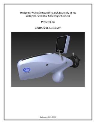
  • 1. February 28th, 2008 Design for Manufacturability and Assembly of the endogo® Palmable Endoscopic Camera Prepared by: Matthew R. Ostrander
  • 2. 2 of 102 Table of Contents 1. Executive Summary.........................................................................5 2. Overview...........................................................................................6 3. Background.......................................................................................6 4. Goal ..................................................................................................10 4.1. Re-design Recommendations Based on DFMA Analysis .................................... 10 4.2. Manufacturing Process (Activity Flow and Production Floor Layout) Design 10 4.3. Extend®-based Process Model................................................................................. 10 5. Problem Definition.......................................................................11 5.1. Metric Definition........................................................................................................ 12 5.2. Discussion of Metrics Selected................................................................................. 17 6. Results..............................................................................................18 6.1. Extend® Process Model (Baseline Design)............................................................. 18 6.2. DFMA Considerations .............................................................................................. 23 6.2.1. Part-Count Reduction............................................................................................ 23 6.2.2. Product Design for Manual Assembly................................................................ 24 6.2.3. Material and Process Selection............................................................................. 33 6.3. Assembly Process....................................................................................................... 37 6.4. Extend® Process Model (New Design)................................................................... 37 7. Summary of Results......................................................................45 7.1. Recommended Design Changes Based on DFMA Analysis ............................... 49 7.2. Recommended Assembly Process for New Design.............................................. 49 7.3. Extend® Model of New Design............................................................................... 49 7.4. Deliverables Checklist............................................................................................... 49 8. References.......................................................................................52 9. Appendices .....................................................................................53
  • 3. 3 of 102 List of Appendices Appendix A – Metric Definitions ............................................................................................ 53 Appendix B – OWC Definitions............................................................................................... 54 Appendix C – Bill of Materials................................................................................................. 55 Appendix D – Probability of Defect Look-up Table ............................................................. 58 Appendix E – Part Attribute Descriptions ............................................................................. 59 Appendix F – Part Count Reduction....................................................................................... 60 Appendix G – Process Time Estimates ................................................................................... 63 Appendix H – Plant Floor Layout ........................................................................................... 81 Appendix I – Material Candidates .......................................................................................... 84 Appendix J – Manufacturing Material and Process Selection............................................. 88 Appendix K – Extend® Models............................................................................................... 95 List of Tables Table 1-1 – Summary of Results................................................................................................. 5 Table 5-1 – Metric/Order Winning Criterion Weighting Matrix........................................ 13 Table 5-2 – Metric Prioritization Determination.................................................................... 15 Table 5-3 – Selected Metrics...................................................................................................... 16 Table 6-1 – Inventory Turns and Cycle Time of the Baseline Design................................. 23 Table 6-2 – DFA Index............................................................................................................... 31 Table 6-3 – Quality..................................................................................................................... 32 Table 6-4 – Derived Parameters............................................................................................... 34 Table 6-5 – Final Polymer Candidates .................................................................................... 36 Table 6-6 – Inventory Turns and Cycle Time......................................................................... 40 Table 7-1 – Inventory Turns and Cycle Time Comparisons ................................................ 50 Table 7-2 – Quality Comparison .............................................................................................. 50 Table 7-3 – Distance Comparison ............................................................................................ 50 Table 9-1 – Metric Definitions .................................................................................................. 53 Table 9-2 – OWC Definitions.................................................................................................... 54 Table 9-3 – Bill of Materials ...................................................................................................... 55 Table 9-4 – Probability of Defect Look-up Table................................................................... 58 Table 9-5 – Initial Material Type Candidates......................................................................... 84 Table 9-6 – Screening of Initial Material Type Candidates .................................................. 85 Table 9-7 – Screening of Polymers........................................................................................... 87 Table 9-8 – Operation Times for Baseline and New Designs ............................................ 100
  • 4. 4 of 102 List of Figures Figure 3-1 – A rigid endoscope (A= eyepiece, B= distal or viewing end) ........................... 7 Figure 3-2 – A flexible endoscope.............................................................................................. 7 Figure 3-3 – Endoscopy “system” or “cart” ............................................................................. 8 Figure 5-1 – CAD Model of the endogo®............................................................................... 11 Figure 6-1 – Baseline Extend Model: Initial Steps ................................................................ 19 Figure 6-2 – Baseline Extend Model: Final Steps.................................................................. 22 Figure 6-3 – Normality Test of Assembly Times................................................................... 27 Figure 6-4 – Normality Test of the Log of Assembly Times ................................................ 28 Figure 6-5 – Assembly Time Pareto Chart.............................................................................. 31 Figure 6-6 – Baseline Extend® Model Output....................................................................... 41 Figure 6-7 – New Design Extend® Model.............................................................................. 43 Figure 9-1 – Plant Floor Layout, Baseline............................................................................... 81 Figure 9-2 – Plant Floor Layout, New Design........................................................................ 82 Figure 9-3 – Model Initial Phase and Steps 1 through 5....................................................... 95 Figure 9-4 – Model Steps 6 through 17 ................................................................................... 96 Figure 9-5 – Model Steps 18 through 29 ................................................................................. 96 Figure 9-6 – Model Steps 30 through 38 ................................................................................. 97 Figure 9-7 – Model Steps 39 through 47 and Data Collection Blocks................................. 97 Figure 9-8 – Model Steps 48 through 59 ................................................................................. 98 Figure 9-9 – Model Steps 60 through 71 ................................................................................. 98 Figure 9-10 – Model Steps 72 through 76 ............................................................................... 99 Figure 9-11 – Model Final Phase.............................................................................................. 99 List of Equations Equation 1 – Inventory Turns .................................................................................................. 19 Equation 2 – Order Size............................................................................................................. 20 Equation 3 – DFA Index............................................................................................................ 24 Equation 4 – Basic Assembly Time Estimation, Alternative 1............................................. 25 Equation 5 – Basic Assembly Time Estimation, Alternative 2............................................. 26 Equation 6 – Probability of Defect (One Operation)............................................................. 32 Equation 7 – Probability of Defect (Entire Assembly).......................................................... 32 Equation 8 – Dimensionless Ranking...................................................................................... 34
  • 5. 5 of 102 1. Executive Summary This document proposes a plan for redesign of the endogo® portable endoscopic camera by applying design for manufacturability and assembly principles and manufacturing process redesign. A baseline and new design were compared across four metrics. These metrics were selected by first defining the critical order-winning criteria (OWC) (those criteria that, if met, will “win” product orders). Those influencing OWC most are shown here. Table 1-1 – Summary of Results Baseline Design Target New Design Inventory Turns 10.9  30 107 Quality, ppm 190,000 ≤ 44,000 10,000 Distance, ft. 25,500 ≤ 5,000 4,840 Cycle Time, min. 280 ≤ 120 112i Inventory turns were calculated via manufacturing process modeling and simulation. The baseline process was modeled using time estimates from the assembly process. The new design was modeled using the reduced process steps arising from design for manufacturability and assembly (DFMA). The model outputs the number of cameras produced in one year and the average daily inventory for that year. The quotient of these two values is the inventory turns. Application of DFMA principles decreased the number of assembly steps and average time per step thereby reducing cycle time. In addition to cycle time reduction, the declining time per step and number of operations contribute to quality improvement. Quality is calculated quantitatively via formulaic approximation consisting of the variables ‘process step quantity’ and ‘average time per step.’ Distance was reduced by adjusting the material flow through the plant. In addition to path distance reductions, because the distance is calculated by summing all distances for all subassemblies, part count reduction also contributed to distance reduction. Finally, plastics manufacturing was a factor contributing to cycle time and poor quality. The material choice was optimized with respect to cost and durability and the appropriate manufacturing process was determined. Polypropylene, a durable, low- cost and temperature resistant material was chosen through dimensionless ranking. This selection led to injection molding as the manufacturing process. The recommended design changes will exceed pre-defined targets, improving device quality and delivery reliability and reducing lead time and cost.
  • 6. 6 of 102 2. Overview Endoscopy is a broad term used to describe examining the inside of the body using a lighted, flexible or rigid instrument called an endoscope. In general, an endoscope is introduced into the body through a natural opening. Thus for these types of endoscopic procedures, the endoscopist (user of the endoscope) is performing an examination of a portion of the body which, without a surgical procedure or autopsy, could not be examined. Endoscopes are used every day by many medical professionals to perform what could be considered a “routine” exam as it pertains to their specialty. Today, video and still photos are captured from the endoscope using relatively large, cumbersome systems of equipment. The endogo® is a compact version of the very large, stationary endoscopic systems that exist. It provides all of the functionality of the state of the art systems with the additional benefit of portability. Design for manufacturability and assembly (DFMA) implies two activities. Both manufacturing and assembly are addressed. Manufacturing is the process of building a part from raw materials. Assembly is the process of mating the parts that have been manufactured into the final product. Therefore, DFMA is that activity of designing a product for ease of manufacturing the parts and assembly of those parts. This document proposes a plan for the redesign of the endogo® portable endoscopic camera by applying DFMA principles. Additionally, presented here is a manufacturing process plan of the redesigned device. The company employed to design and produce the endogo® is BC Tech, Inc. based in Santa Cruz, California. The company with the patent on the endogo® is Envisionier Medical Technologies, LLC based in Gaithersburg, Maryland. Dr. Patrick Melder is Envisionier’s founder and CEO. Dr. Melder will serve as the company liaison. 3. Backgroundii Endoscopes have literally revolutionized the practice of medicine over the past two decades. While crude endoscopes have been used for nearly a century, it has not been until the last 50 years that endoscopes have been able to produce brilliant images which have aided the endoscopist in visualizing body orifices and body cavities. In 1965 the Hopkins rod lens system, illustrated in Figure 3-1, was developed by Karl Storz Endoscopy. This system was an advance over the “tube” with lenses on each end with air between the lenses. The Hopkins system, which is still in use today, is a series of glass rods at intermittent distances from each other sheathed in a tube. The result is a much more brilliant image, a brighter image (with accompanying fiber-optic light source), and a wider field of view.
  • 7. 7 of 102 Figure 3-1 – A rigid endoscope (A= eyepiece, B= distal or viewing end) The preceding describes a “rigid” system. These endoscopes are straight, rigid instruments which can be damaged and even broken if bent beyond tolerances. Understandably, a rigid instrument will not do well within the confines of the esophagus, intestines, or trachea/bronchi (breathing tube). For visualizing these structures, a “flexible” endoscope is available which is composed of tiny fiber-optic glass rods which simply transmit an image from the tip to an eye piece. Another bundle of fibers is used to carry the light so the object being visualized is illuminated (see Figure 3-2) While flexible endoscopy allows for the ability to “look around corners” it limits the endoscopist’s ability to perform complex procedures. Biopsy and limited procedures can be performed using a flexible system. However, the greater value of a flexible endoscope is generally for diagnostic purposes. These are used by a host of medical specialists including surgeons and non-surgeons. Figure 3-2 – A flexible endoscope The scopes by themselves serve as valuable tools in diagnoses and medical procedures, but they are incapable of archiving images for recall later. Currently this functionality is provided by way of additional equipment. These endoscopic visualization “systems” or “carts” contain a light source, a camera head, a camera control unit (CCU), and a monitor. If the user wishes to capture, store, and edit the images and/or video, then additional equipment must be purchased such as a tape recorder (VHS or DV)/optical media device and a printer. These systems are large (see Figure 3-3) and quite common in large academic institutions in the examination rooms of the specialists who would A B
  • 8. 8 of 102 use them. Additionally, every hospital in the U.S. and any in the world performing endoscopic surgery would have a system like this for visualization. Figure 3-3 – Endoscopy “system” or “cart” These tower systems are very expensive and usually only purchased by hospitals and large teaching institutions. In general, the private practitioner will not purchase such expensive equipment unless he/she can bill for the service and justify the cost of the system. For millennia, the medical physician has relied on the written word and pen and paper to describe or draw what he/she saw during an examination. While this remains adequate, as technology becomes more usable and less expensive it will find its way into a private practice setting. With the advent of digital cameras in the mid-nineties, many saw an opportunity to take digital technology and incorporate it into medical practices. This, though, was not an easy task. First, Dr. Melder wanted to accomplish this as inexpensively as possible. At the time, digital single lens reflex (SLR) cameras were available but cost thousands of
  • 9. 9 of 102 dollars. And the techniques of using a 35mm SLR camera for endoscopic photography were not known. In order to do this inexpensively, Dr. Melder took an off the shelf Canon PowerShot G1 and attempted to find equipment to which endoscopes could be adapted. After a failed attempt, he found Precision Optics [10]. They were able to supply an endoscopic coupler so he could take digital still photos. However, the problem with off-the-shelf digital cameras is that no two are alike and even subsequent models of the same line may be re-designed so that previously purchased equipment may not fit. This presents a problem when trying to introduce new techniques or technologies. This hindered Dr. Melder’s second goal of a “standard” solution like that of the SLR legacy system. If, for example, a user had an Olympus camera body, he/she could easily switch to using a newer camera from Nikon because the lenses and adapters had a “standard fit.” Third, Dr. Melder wanted to accomplish what no manufacturer has been able to accomplish to date and that is extreme portability so that the same great images available in the operating room and clinic are available in the hospital ward or in the emergency room during consultation. The proposed technology (FireWire portable digital endoscopic camera) is a unified solution, meeting Dr. Melder’s requirements. The idea is to provide a device that can be used anywhere without being tied to a proprietary platform: to take what is commonly found in the consumer digital camera market (extreme functionality and ease of use) with what is found in endoscopy (a need to produce high quality diagnostic and therapeutic video and still imagery) in differing environments. In effect, what is needed is a small, compact, digital endoscopic imaging device, ergonomically designed to provide maximal comfort for short and prolonged use. The proposed device would have a universal endoscopic coupler to accommodate standard endoscopes. It would be designed with zoom and focusing capabilities. The camera would allow the user to control image quality. It would have on board and removable storage media. It would have a light and long-lasting rechargeable battery. The device would have an optional liquid crystal display flip screen for viewing images, or would use current high speed data transfer (IEEE1394 or FireWire) for live image acquisition and transfer to a Macintosh- or Windows-based computer. And it could be used with current off-the- shelf TV monitors for viewing images. It is this concept that drove the design of the endogo®. While the current design meets the functional needs, no consideration was given to the device’s manufacturability during design. This was due to the desire to introduce the product to the market promptly. The following sections define the next step in the evolution of the endogo®.
  • 10. 10 of 102 4. Goal The goal of this effort was to recommend design and assembly process changes that will enable production of the endogo® at reduced cost, increased speed and higher quality. This project has resulted in a reduction of part count and more efficient, faster assembly. DFMA principles were applied and their effectiveness was demonstrated by comparing key performance metrics taken from the current production system and an Extend®iii-based model of the new system. The medium through which the goal was achieved are the three products presented below. Those three necessary products are then carried through the entire document and linked to a set of specific performance criteria. The rationale for each of the products below and their relevance to the stated goals is described later in this document. The following sections are only a summary of the products. 4.1. Re-design Recommendations Based on DFMA Analysis The re-design recommendations arose first out of part count reduction analysis (the rationale for this process and its relevance to the stated goals is described later). These were then refined based on information gained from assembly time and probability of defect calculations. Those design recommendations that demonstrated the greatest potential for design impact were prioritized higher for the purpose of controlling scope. A subset of the finalized design recommendations were further reviewed using a material and manufacturing process selection. Namely, those parts that are currently machined or are being produced using “soft” tooling were analyzed for the purpose of determining a more cost-effective manufacturing approach. 4.2. Manufacturing Process (Activity Flow and Production Floor Layout) Design Once the new design was determined from the DFMA analysis, the production floor layout and the activity flow were designed. The production floor layout for both the baseline design and the new design were used to estimate part acquisition times. These estimated part acquisition times, in conjunction with the estimated assembly times were used to calculate the DFA Index, a number that quantifies assembly performance. 4.3. Extend®-based Process Model The assembly and part acquisition times estimated for the new design were used in developing an Extend®-based model that was used to optimize the process, i.e., minimize the cycle time and reduce WIP.
  • 11. 11 of 102 5. Problem Definition The nature of this effort was to produce a high quality, compact endoscopic camera for highly frequent use in a variety of medical environments. Quality is critical given the nature of the medical field and frequency of use. Production rates are estimated but subject to fluctuation. The camera is small and comparatively simple. The assembly process currently involves organic and vendor-supplied subassemblies. The endogo® Palmable Endoscopic Camera (Figure 5-1) is the name given to the camera which has recently completed the design phase and has now begun initial production. The camera will be considerably smaller than anything available today. As presented previously, the concept is to take commonly available technology and integrate it into a system that offers portability, something current models cannot provide. Figure 5-1 – CAD Model of the endogo® BC Tech arrived at the current design (Figure 5-1) under strict budget and funding constraints. These constraints required use of commercial-off-the-shelf technology and a design approach focusing primarily on performance. Design for manufacturability and assembly was not considered. The bill of materials (BOM) (Appendix C) for the current design served as a point of departure for this effort. Housing LCD Coupler (endoscope attaches here) Rotates Coupler Assembly Main PCB Secondary PCBs Battery USB
  • 12. 12 of 102 As stated in the Goals section, a key consideration was part count reduction. The BOM establishes the baseline from which progress can be measured with respect to part count. This project will accept the current design and BOM as they exist and propose a more manufacturable, de novo design. 5.1. Metric Definition The previous section laid out the desired end-state (goals) and the method to get to that end-state (the three “products”). In order to establish criteria for goal achievement, several metricsiv were developed in order to define the problem quantitatively. The remainder of this section is devoted to explanation of how those metrics were defined. These performance criteria indicated if the goal stated previously was met. Therefore the goal states what was to be accomplished, the products defined the medium through which the goals were achieved and the metrics were the standards used to determine whether or not the goals were met. The first metric defined was the cycle time. After production initiation Envisionier’s business model assumes that a minimum of 230 units will be produced within the first year. Given the strength of the initial response, e.g., the establishment of agreements with two European distributors and likely establishment with one US distributor, that number has likely doubled. For conservatism, initially it was assumed that 4 times that amount (~1000 cameras per year) will be required in the initial years of production. Assuming 250 work-days per year, 8 hours per day, and a single production line, the minimum required cycle time will be 120 minutes. This metric was derived from the projected demand and was not derived directly from any of the previously stated goals. The remaining metrics were devised with the intent of supporting goal achievement. In addition to the cycle time, several other metrics were established to serve as guides for production. In order to simplify the approach, criteria were established for defining the most vital metrics. The concept of order-winning criteria (OWC) was chosen in order to vet the candidate metrics [14]. An OWC is defined as the minimum level of operational capabilities required to get an order. For example, the primary OWC for an airline ticket is typically price. Given the relative consistency of service and leg room across the range of alternative airlines, most people simply choose the cheapest flight. Of course, there are limits to this concept. Few people, if any, would pay $5 to ride in the cargo hold. While comfort is not the driving OWC, it is simply a lower priority OWC. Therefore, there are many OWC for any given product, but some of them hold priority over the others. Furthermore, for many products, they are dynamic, i.e., they will change as the market matures. Typical OWC (and those chosen for this effort) include price, quality, lead time, delivery reliability, flexibility, innovation ability, size and design leadership. Definitions for each of these are provided in Appendix B. Those most applicable to the
  • 13. 13 of 102 endogo® were selected and weighted as indicated in Table 5-1. The OWC are not necessarily items that can be altered directly by the manufacturing processes. Rather, they are affected by measurable quantities that can be directly manipulated within the manufacturing process. For example, the price cannot simply be chosen by those designing the manufacturing process. Rather, the price is determined by how efficiently the product can be produced. The measures determining how a product performs in the various OWC are referred to here as “metrics.” Table 5-1 depicts which OWC are affected by which metrics. For example, Table 5-1 indicates that an improvement in Set-up Time will improve performance in the price and lead time OWC, an improvement in Quality will result in improvement in the price and quality OWC, etc. Table 5-1 – Metric/Order Winning Criterion Weighting Matrix Metrics OWC Set-UpTime Quality SpaceRatio Inventory Flexibility Distance Uptime Weight Price        1 Quality        10 Lead Time        1 Delivery Reliability        2 Flexibility        0 Innovation        0 Size        0 Design Leadership        0 As indicated in the ‘Weight’ column (Table 5-1), flexibility, innovation, size and design leadership were eliminated by assigning a weight of zero to those criteria. Flexibility, the first OWC eliminated, is the measure of the capability to produce multiple parts per machine. Given that the endogo® is the only product currently being developed by Envisionier, this metric is irrelevant for this process because the ability to produce many parts by one machine is unnecessary. Furthermore, very few subassemblies are manufactured in the BC Tech facility in Santa Cruz. Given that, having highly flexible machining equipment is unnecessary.
  • 14. 14 of 102 Innovation is not a consideration because there is nothing manufacturing can do to affect that OWC. The same is true of design leadership. The final OWC eliminated, size, is more a function of ergonomics than performance. The camera can only be so small because it must fit comfortably in one’s hand. Further, in comparison to state–of-the-art endoscopic units, this device is exceedingly small. And it must be, because that feature is one quality that permits it to be truly portable. It is the endogo’s® portability that distinguishes it from all other endoscopic cameras available. Therefore, any attempt to further reduce the size would not deliver proportional returns on the device’s value to the customer. That leaves only four OWC with relevance. Quality was weighted the highest. Quality is imperative primarily because of the environment in which this device will be employed and because it is directly linked to the goal statement in the previous section. It will be used at regular intervals throughout the day for several days on end. It must stand up to the demanding clinical environments. A device that malfunctions in a medical environment quickly becomes marked as unreliable, thereby significantly reducing its marketability. Delivery reliability was weighted second in importance, though significantly lower than quality. The ability to meet customer requirements in a timely manner is important, but initially it is considerably less important than producing a quality product. It is also linked to the goal statement previously in that it is one criterion that indicates the speed with which the device can be manufactured. Price was ranked third. That is because of the wide margin between what the endogo® costs to manufacture and the purchase price of current models with similar functionality. The purchase price of current models is upwards of $60,000. Less expensive “budget” systems are available from $8 – 12,000. The endogo’s® initial target cost to manufacture is $1,000. This wide profit margin makes the cost of manufacturing the device of less concern initially. However, as competitors enter the market, it will be advantageous to be in a position to set a purchase price that is below what any entrant could approach. This fact and the linkage to the goal statement lead to its inclusion in the OWC. Finally, lead time was weighted the same as that of price. Lead time is of lesser importance due to the fact that doctors that will purchase the endogo® have been functioning without it for some time. Therefore, a wait for the product will not create a dire circumstance. However, like price, as the market matures, this OWC will increase in importance and is therefore important to receive some weighting greater than zero.
  • 15. 15 of 102 Table 5-2 – Metric Prioritization Determination Weighted Scores Set-Up Time Quality SpaceRatio Inventory Flexibility Distance Uptime Price 1 1 1 1 1 1 1 Quality 0 10 0 10 0 10 0 Lead Time 1 0 0 1 1 0 0 Delivery/Reliability 0 0 0 2 0 0 0 Flexibility 0 0 0 0 0 0 0 Innovation 0 0 0 0 0 0 0 Size 0 0 0 0 0 0 0 Design Leadership 0 0 0 0 0 0 0 Totals 2 11 1 14 2 11 1 With a set of OWC in place, how they interact with the metrics may now be determined. Given the weighting scheme, Table 5-2 indicates that the highest priority metrics were Inventory Turns, Quality, and Distance. The metrics selected, in addition to cycle time (calculated previously), are summarized in Table 5-3.
  • 16. 16 of 102 Table 5-3 – Selected Metrics Metric Weighted Score World Class Redesign Target Design Changes Required Inventory 14  1000 turns  30 turns Reduce Average Daily Inventory by 6 Times Quality 11 Captured: ≤ 1500 ppm Warranty: ≤ 300 ppm Captured and Warranty: ≤ 44000 ppm Reduce Steps and Time per Step by Half Distance 11 ≤ 300 feet ≤ 5000 feet Reduce Distance Traveled by One Part by 20% and Part Count by Half Cycle Time – – ≤ 120 minutes Reduce Part Count by Half and Time per Step by Half
  • 17. 17 of 102 5.2. Discussion of Metrics Selected Inventory received the highest possible score under the metric selection scheme presented previously. An inventory “turn” is a measure of how efficiently inventory is turned into product. Inventory Turns are calculated by dividing the annual cost of goods sold by the daily average inventory value. Therefore, it is a measure of how often the entire inventory is “turned” over in a year. Low Inventory Turns are indicative of inefficient manufacturing processes. The implementation of “lean” manufacturing processes is directed primarily at cutting out the inefficiencies in the flow from raw material to finished product. A more efficient flow, which avoids unnecessary WIP and stock, reduces wasted time and material. Therefore, it is relatively simple to see how Inventory Turns affect price in that the amount of resources expended per finished product is minimized, thereby maximizing the profit margin allowing the producer to under-price competition. Furthermore, delivery reliability is enhanced because efforts to increase Inventory Turns lead to simplified systems with fewer “moving parts,” i.e., variability in the production process is reduced as complexity is reduced. As unnecessary and wasteful processes are eliminated, the opportunity for variability reduces and delivery reliability is improved. Additionally, lead time is also affected by efforts to increase Inventory Turns because the reduction in wasteful processes increases the responsiveness of the system as a whole. A less obvious connection to the metric of Inventory Turns is that of quality. Inventory is an indicator of quality in part because as assembly time increases for a given product, the likelihood of poor workmanship increases as well. Barkan [2] points out that there is a strong, directly proportional correlation between the DFA time estimate per operation and the average assembly defect rate per operation. Therefore, more efficient assembly processes requiring less time not only lead to reduction in WIP, thereby increasing Inventory Turns, it also leads to higher quality. Table 5-1 indicates that the metric Quality affects the OWC of quality and price. As a point of clarification, the metric “Quality” is a specific, quantifiable value whereas the OWC “quality” is more qualitative and a method of communicating product marketing strategy throughout an organization. For instance, if the OWC of quality is given priority over all other OWC within an organization, all facets of that organization know that the consumer is primarily concerned with that aspect of the product when comparing it to other products in the market space. To the manufacturing department within that organization, this overarching product strategy translates to a need to focus on the metric of Quality. In doing so, the metric of Quality will directly impact the OWC of quality by reducing the number of faulty products. In addition, the OWC of price will also be affected because re-work (wasteful activity) is eliminated, which is another means of reducing the amount of resources expended by the organization to arrive at a finished product. The metric of Distance, like Quality, affects the OWC of quality and price. Distance is the actual distance traveled within the plant as it moves from raw material to final
  • 18. 18 of 102 product. This metric is indicative of the degree to which the product is handled within the manufacturing and assembly plant. Generally, the more a product is handled, the greater the probability of defects [14]. Furthermore, price is affected because distance is indicative of the amount of non-value-added time that the product spends within the plant. This non-value-added time translates into greater resources expended per product and therefore a higher consumer price for a given profit margin. Cycle time is more a constraint of the system than a metric because it was calculated based on projected demand. It does, however, also affect quality, price, delivery reliability and lead time. While the metric is necessary for status monitoring based on product demand, it is interdependent with and redundant to all of the previous metrics and served as a supporting metric, verifying their progress. 6. Results In order to drive toward the OWC described previously, activities were oriented toward achieving the stated metrics. The approach was therefore to devise tasks that result in achievement of the metrics. It is these tasks that produced the three products listed in the “Goal” section. The metrics defined previously assisted in determination of goal achievement by measuring the products against them. Before continuing, some terminology must first be clarified. The terms manufacturing and assembly are not interchangeable. Manufacturing refers to the process of producing a finished subassembly from raw material. Assembly refers to the aggregation of subassemblies, ultimately into a finished product. Both manufacturing processes and assembly processes were addressed by this project, but to varying degrees. Not all subassemblies were analyzed from a manufacturing perspective, and only the final assembly within the facility at which the final product is produced was considered. 6.1. Extend® Process Model (Baseline Design) The first task was to model the baseline process in Extend®. Initiating the process in that manner was beneficial for two reasons. First, it enabled clear understanding of the baseline design processes. That understanding better facilitated process modification. A thorough understanding of the manufacturing and assembly process led to intelligently selected design choices. Second, the model assisted in estimation of Inventory Turns. Using the model, the necessary information used to calculate Inventory Turns were generated. The necessary information includes the average daily inventory (including both stock and WIP) and the cost of goods sold in a year. The equation for Inventory Turns is provided below.
  • 19. 19 of 102 $, $, InventoryAverageDaily AnnuallySoldGoodsofCost TurnsInventory  (1) Equation 1 – Inventory Turns The same calculation was done for the new design and the two were compared in order to understand how design changes have improved the process. The model consists of three fundamental parts. The first section simulates demand, orders material based on subassembly lead time and endogo® lead time and regulates the number of cameras worked on simultaneously. This section is illustrated in Figure 6-1. Figure 6-1 – Baseline Extend Model: Initial Steps First, demand is simulated by a triangular probability distribution with the high and low values at plus and minus 10% of the most likely value of 120 minutes per camera demanded (). This assumes a demand of 1000 cameras per year (see Section 5.1) at 120,000 minutes per year. The 10% variation from that demand is used to represent realistic demand and is loosely based on current trends, though the product is not mature enough to accurately predict demand fluctuation. While demand is important in deriving Inventory Turns (the primary purpose of the model), this model is intended as a comparison tool between the new design and the baseline design, given identical market conditions. Another purpose for the model is to simply determine if the production line is capable of meeting the predicted demand as determined in Section 5.1. Therefore, as long as the simulated market conditions are equivalent between the new model and the baseline model and the average estimated demand is realistic (as derived in Section 5.1), the demand parameter as defined will support the requirement to serve as a basis for comparison between the two systems and provide a means of determining if the process can produce the required number of cameras.    
  • 20. 20 of 102 The next step () in the model is to simulate purchase of materials for production. There are two considerations when purchasing materials. The first consideration is whether there is sufficient demand to commit to material purchase. The model does not allow material to be purchased until at least the number of cameras worked on simultaneously is in demand. For the baseline design, this number is 10. BC Tech reasoned that efficiencies can be realized by an individual technician working on multiple cameras at the same time. The number they chose was 10. Therefore, the baseline model uses 10 as the number of cameras worked on simultaneously. That defines the minimum number of cameras for which parts are ordered. The maximum number is determined in this system by (2). TimeLeadendogo TimeLeadySubassembl SizeOrder  v (2) Equation 2 – Order Size where, Subassembly Lead Time (Time per Order)  The longest time in minutes that any subassembly takes to be ready for assembly from the time it is ordered and, endogo Lead Time (Time per Camera)  The average amount of time required to build one camera.vi Observe that the result of (2) is in “Cameras per Order.” This provides the maximum desired amount of material on hand given a particular endogo and subassembly lead time. If more than this amount is ordered, it will be more than can possibly be worked on before another order must be made. If less than this amount is ordered, it will result in a delay in production. Take the following as an example: For simplicity, assume that a product has a subassembly lead time of 100 days and a production lead time of 10 days. The process would go as follows: 1. Materials are ordered on Day 0. 2. Materials arrive on Day 100. 3. Production begins and materials are ordered for the next lot at the end of Day 100. 4. On Day 200 the first lot will be complete and 10 cameras will have been built. Also, the materials ordered at the end of Day 100 will arrive just as the first 10 are completed so that the next lot can be produced. 5. Finally, materials for the next lot would be ordered at the end of Day 200 and will arrive when the next 10 cameras are complete.
  • 21. 21 of 102 Assuming demand meets or exceeds production capacity and we do not want any more material on hand than we need, it would be optimum for materials to arrive for the next lot the moment after we finished the first lot, so as to limit inventory. If endogo® Lead Time and Subassembly Lead Time remain relatively constant, the number of cameras produced within a Subassembly Lead Time determines the amount of material to purchase for the next lot. The number of cameras produced within the Subassembly Lead Time is determined by (2). For the baseline system, the Subassembly Lead Time is six weeks (14400 minutes). For each camera, the endogo® Lead Time is calculated and the average of those values is used in the Order Size calculation in (2). The camera material purchased is stored in a queue immediately after the gate (). The size of this queue is stored as a value called “Stock.” This is one part of the inventory of the entire system. After this point in the model, only the number of simultaneous cameras worked on (in the baseline case this value is 10) are allowed into the process. Also, only one camera is worked on at a time and all 10 cameras pass through a given step before moving on to the next. This simulates the process BC Tech uses. In that process, there is one technician assembling 10 cameras at a time, taking each camera through one step at a time. After this initial phase, the cameras enter the 76 steps in the process and all of the cameras being worked on simultaneously are passed through each step until it reaches final inspection. Each of these steps is based on estimates from BC Tech for actual assembly time. Again, variation in process times was modeled using a triangular probability distribution with the maximum and minimum values at plus and minus 10% of the most likely value, respectively. These probability distributions are estimates used to enhance the model’s realism. In addition to the 76 steps in the process, a step for “pre-work” is included. The pre-work time was estimated at 83 minutes and included modification of the cast plastic parts by hand. Within these 76 steps, the cameras are counted as WIP until they are “shipped” after passing final inspection and leave the plant. The third and final phase of the process is final inspection and rework and is illustrated in Figure 6-2. The first step is to determine if rework is required. The “DE Eqn” block leading this section () first uses a uniform distribution in order to determine if rework is required. The value used for the likelihood that rework is required is 19% as calculated by estimating the Quality, which is subsequently presented. If the camera does have a defect, a triangular distribution with minimum, maximum and most likely values of 30, 120 and 60 minutes respectively determines the amount of time spent on that work. These values are estimates from the technician performing the re-work.
  • 22. 22 of 102 Figure 6-2 – Baseline Extend Model: Final Steps After any final re-work that may take place, the camera is ready to ship. At this point, one key consideration for this study must be examined. The model does not take into account the time the cameras spend in transport from BC Tech to Envisionier. The intent of this study was to assess the capabilities of the plant itself. Including shipping time effectively adds one step to the process of 1 day (480 minutes). This does prove to be a key consideration, especially when faulty product is discovered after the product has been shipped to Envisionier. If that occurs, the product must be shipped back to BC Tech for rework, adding not only the rework step but also the shipping time to send it back. The inclusion of shipping time does affect inventory significantly. It highlights the importance of proximity of the production plant relative to the customer as well as the importance of warranty quality (defects that are found after shipping). However, the purpose of this study is to evaluate the effectiveness of the plant itself. In order to do that, the inventory is limited to the stock and WIP located on site at the BC Tech facility. When the camera leaves the plant, the endogo Lead Time is recorded by simply subtracting the time it leaves from the time it entered the process (). The lead times are recorded and averaged for use in the Order Size calculation discussed previously. In the next step, “GATE” () is set to a value of “1” when 10 cameras have left the process. This allows 10 new cameras to enter the process (see Figure 6-1), but not before “WIP RESET” is set to a value of “1” causing “IN PROCESS” (the number of cameras being processed) to be reset to a value of “0.” After this, 10 new cameras enter the process and “RESET” is set to a value of “1” causing “THE DEPARTED” (the number of cameras that have been completed) to be reset to “0.” All of this is to calculate how many cameras are in process at any given moment and to only allow one camera to be worked on at a time (because there is only one person working on them).    
  • 23. 23 of 102 Finally, the cameras exit the process and they are counted (). Each simulation is run for one year (120,000 minutes). The number of cameras produced, the Cycle Time, the Inventory Turns, and the average daily inventory are calculated. The values of interest for this study are the Inventory Turns and the Cycle Time. The model was run 30 times and the following values were determined: Table 6-1 – Inventory Turns and Cycle Time of the Baseline Design Metric Average Upper Bound (99% Confidence) Lower Bound (99% Confidence) Inventory Turns 10.9 11.0 10.8 Cycle Time, min 278 387 169 The Cycle Time compares well to observed performance from BC Tech. A typical week would produce between 8 and 10 cameras which translates to a five to four-hour cycle time. The model predicts 4.6 hours per camera. The reason for the large confidence interval is that cameras are produced 10 at a time. Therefore, 10 will be produced in rapid succession, spaced out only by the duration of the last step. That is followed by a long waiting period until the next round of 10 is produced, thus producing a wide range in Cycle Time. Clearly, the baseline will not meet the requirement of 120 minutes per camera. 6.2. DFMA Considerations The second task was to analyze the design with respect to DFMA considerations. The design goals initially did not involve primary emphasis on manufacturability or assembly in order to keep up-front costs low and for rapid market entry. Therefore, the current design, while functional, is not optimally designed for manufacturability and assembly. The design changes recommended as a result of this study will be implemented in a de novo design that is more cost effective to produce and higher quality. While materials and DFMA were considered for various subassemblies, the process times for manufacture of those subassemblies were not considered in the process model. The DFMA-related considerations include the following: 1. Part-Count Reduction 2. Product Design for Manual Assembly 3. Material and Process Selection 6.2.1. Part-Count Reduction The first technique employed was that described by Boothroyd [3]. This process involves three rules to be followed each time a new subassembly is added during assembly. Those three rules are presented here:
  • 24. 24 of 102 1. During operation of the product, does the part move relative to all other parts already assembled? Only gross motion should be considered. Small motions that can be accommodated by integral elastic elements, for example, are not sufficient for an affirmative answer. 2. Must the part be of a different material than or be isolated from all other parts already assembled? Only fundamental reasons concerned with material properties are sufficient for an affirmative answer. 3. Must the part be separate from all other parts already assembled because otherwise necessary assembly of other separate parts would be impossible? If all three of the above questions can be answered negatively, the part is a candidate for assimilation to the subassembly to which it is being attached, thereby reducing the overall part count by one. This process is continued for each part as it is added to the assembly. The overall part count was reduced from 86 to 35. The process described previously was applied to each of the 76 steps identified in the process. Each of the changes is detailed in Appendix F. 6.2.2. Product Design for Manual Assembly Once the part count was reduced to the lowest extent possible, the techniques for assembly were then addressed. In general, the goal was to apply design for assembly principles for the purposes of increasing ease of part handling. Specifically, the baseline model was analyzed using design for assembly principles. To that end, the DFA Index, a measure of assembly efficiency, was first calculated. That number was generated by dividing the theoretical minimum assembly time by the actual assembly time. assemblycompletetotimeestimatedt partonefortimeassemblybasict partsofnumberltheoreticalowestN IndexDFAE where ttNE ma a ma maama      min min , / (3) Equation 3 – DFA Index Nmin is the number of parts determined by applying the three rules of part-count reduction. ta is generally assumed to be 3 seconds on average [3]. However in this case ta was originally proposed to be determined as follows:
  • 25. 25 of 102 timeleadtheofdevst designbaselineinpartsofnumberactualN cameraonebuildtorequiredtimeCT where N CT t CT actual actual CT a .. , 282.1        (4) Equation 4 – Basic Assembly Time Estimation, Alternative 1 The numerator of the equation above is defined as the theoretical minimum lead time that could be achieved for the endogo®. 1.282CT reduces the average down to the 10th percentile value of a normal distribution indicating that all cycle times less than or equal to the minimum cycle time, as defined here, would be achieved 10% of the time. ta then represents the average time per operation that would have to be achieved in order for the theoretical minimum cycle time to become the new average cycle time. The justification for this approach is the fact that the numerator of the DFA Index equation, (3), is the theoretical minimum total assembly time of the endogo®. Boothroyd’s [3] estimation technique (estimating the average assembly time as 3 seconds) assumes that there is not actual knowledge of the product’s assembly times because it assumes that these estimates are taking place simultaneously with design. In this case, an actual design is under modification and the theoretical minimum assembly time for each subassembly can be estimated from actual data (The cycle time (CT in (4)) and its standard deviation (CT in (4)) were determined from data acquired from the BC Tech facility.). The reason the 10th percentile approach was taken was that it was desired that the DFA Index provide useful information about how close the actual system is to the ideal. Using actual statistical data in generating the theoretical minimum assembly time would theoretically result in a more realistic estimation of design performance. The 10th percentile was chosen as something that is achievable statistically speaking and not unrealistically ideal. Again, the desire was to define a DFA Index that is achievable yet requiring near-perfect operation. In this way a DFA Index of 1.0 has meaning to designers and is truly a measure of how close the system under consideration is to ideal. Furthermore, this ta is determined based on handling of parts that are typical to this product. The ta of 3 seconds recommended by Boothroyd [3] is an average, ranging across widely varying manual assembly operations. The approach for determination of ta described above was pursued. As it was calculated it was determined that the values being calculated were much higher than would be estimated using the Boothroyd approach. Therefore, the value calculated for the minimum assembly time that could be achieved for the endogo® was higher than the time estimated for assembly using the techniques from Boothroyd. This yields assembly efficiencies higher than one. The first explanation for this is that considerable amount of time was being spent on “pre-“ and “re-work” activities. “Pre-work” was effort that went into the received cast plastics. Most of the plastics were not within tolerance due to limitations of the casting process. This required the technician to
  • 26. 26 of 102 remove excess material by hand prior to beginning assembly. BC Tech estimated that 96 minutes per camera was spent in this type of activity. “Re-work” is work that was done to correct issues with the cameras when they failed final inspection. These two activities are accounted for in the cycle time estimates from BC Tech, but are not included in estimates for assembly time. The problem with this estimate technique was that parts of the data were derived from research and parts were derived from analysis, i.e., the Boothroyd technique. Therefore, the next approach was then to use a comparison of estimates using the Boothroyd technique in lieu of using actual cycle time data. This approach proved more fruitful, resulting in assembly efficiencies that were reasonable. For this approach, the estimates for the assembly times for each step were examined. As (5) indicates, as with the previous method, the 10th percentile is again targeted as a reasonable minimum. steppertimeassemblyestimatedtheofdevst steppertimeassemblyestimatedaveraget where tt estimated averageestimated estimatedaverageestimateda .. , 282.1 , ,      (5) Equation 5 – Basic Assembly Time Estimation, Alternative 2 However, this estimation technique also was discarded because it assumes that the estimated assembly times are distributed normally for a given product. An Anderson- Darling normality test conducted on the data, provided in Figure 6-3, indicates that the data are not distributed normally. Therefore, the second approach was also discarded. However, the log of the data, as indicated in Figure 6-4, is normal.
  • 27. 27 of 102 Assembly Times, seconds Percent 2520151050-5 99 95 90 80 70 60 50 40 30 20 10 5 1 Mean <0.005 7.355 StDev 5.435 N 30 AD 1.967 P-Value Normality Test of the Assembly Times Normal Figure 6-3 – Normality Test of Assembly Times
  • 28. 28 of 102 Log of Assembly Times Percent 1.61.41.21.00.80.60.40.20.0 99 95 90 80 70 60 50 40 30 20 10 5 1 0.411 10 Mean 0.542 0.7733 StDev 0.2824 N 30 AD 0.307 P-Value Normality Test of the Log of Assembly Times Normal Figure 6-4 – Normality Test of the Log of Assembly Times This allowed for the possibility of analyzing the data in the log form and then converting back to assembly times after the basic assembly time is determined. Figure 6-4 indicates that the 10th percentile occurs at 0.411. Converting this number from its log form, it becomes 2.58 seconds. Therefore, on a design of this type, 10% of the time there will be a step that is less than or equal to 2.58 seconds. This number will therefore serve as the theoretical minimum for this design. The significance of choosing the correct ta is that it determines what the “ideal” system for this product would be in terms of assembly time. With something close to what is ideal but achievable, it provides an understanding of the extent to which the design can actually be improved beyond what it is currently. If the DFA Index was near a value of 1 to begin with, investing in improving assembly efficiency would not be valuable time spent. Another benefit of the DFA Index is that it provides a means to compare designs relative to one another in order to determine the design changes’ relevance. When using the DFA Index to compare two designs relative to one another, there is less significance in selecting the correct ta. This is because when the designs are compared to one another, we are simply comparing the estimated assembly times, tma. The average assembly time, ta, and the lowest theoretical part count, Nmin, stay constant.
  • 29. 29 of 102 tma in (3) is an estimate of the entire assembly time. This is based on analysis of the various subassemblies to arrive at an assembly time for each part. Boothroyd [3] provides various handling, assembly and fastening considerations and estimation techniques that were used in determining the estimated time to complete the assembly. The times to execute each step in the assembly process at the BC Tech facility were estimated using the techniques presented by Boothroyd [3]. Given that this study assumes the device is already in production, it would have been possible to extract tma directly from the operations themselves by timing each individual operation. This approach has been rejected based on the fact that we are comparing estimates between the baseline and new designs. The design change recommendations arising from this study will not be implemented as a part of the study. Therefore, only the assembly time estimates of the new design will be known. For consistent comparison of the new and baseline designs, they both should be based on the estimates for processes. In addition to assembly times, the part acquisition times must also be determined. Determining the acquisition times also required that the assembly layout be designed. The technique for assembly design presented by Boothroyd [3] was applied. Boothroyd [3] breaks out the various assembly layouts based on the complexity and size of the device in order to determine part acquisition time. Assembly takes place in an environment where many products other than the endogo® are produced. Therefore, the assembly layout design requires a modular approach, i.e., not specific to this product but flexible enough to keep all necessary subassemblies and tools within reach of the worker. Furthermore, Boothroyd [3] categorizes acquisition times based on the size of the parts. For the assembly procedure in question, all parts are in the smallest size category, which is less than 15 inches. Furthermore, in designing the assembly layout, a primary constraint was the design goal of 5000 feet or less Distance of part motion. In order to reduce the Distance, a few simple revisions in plant operations were incorporated. The first recommendation was to simply arrange each of the functions sequentially in the order they typically occur. Further, receiving and inspection will now take place in the same location by the same person. A cubicle previously unused was turned 180 and made into the receiving/inspection station. Then the receiving rack was moved to be directly adjacent to the receiving/inspection station. The last change was to move the endogo® workstation next to the receiving/inspection station in the warehouse. This change was necessary to meet the design goal of 5000 feet. Additionally, as none of the parts in the new design will require machining, the distance traveled to the machine shop has been removed entirely. Appendix H provides an illustration of the plant floor layout and process flow for the baseline and new design. The layout as shown in Figure 8-2, Appendix H, requires 4840 feet.
  • 30. 30 of 102 The next adjustment has to do with the work station itself. The current practice is to contain all of the parts in a rack at a location about 13 feet away from the work station. They then “kit” each camera so that all of the necessary parts are in the same bin at the work station. They work on 10 cameras at a time so that the material for 10 cameras remains at the work station. This practice is unnecessarily cumbersome. The “kits” cause the technician to have to search through the bin in order to find the particular part he/she is looking for. Rather than “kitting” the cameras it is recommended that all of the parts be relocated from the storage rack to the actual work station. The work stations are outfitted with shelves that can be used to store the parts. With the reduction in parts of the new design, all of the parts would fit at the work station. This change eliminates the need for a storage rack altogether, freeing up space. It also eliminates the need for “kitting” cameras so the technician does not have to move back and forth between the work station and the storage rack. This then eliminates the process of searching through the kits for the appropriate part. Also, each part bin should be arranged in the order of assembly with a label indicating the step number, part number and a picture of the part making it easy to locate the correct bin. Once the time to assemble (tma) was estimated, those parts that require the most time were aligned with the areas of potential design simplification identified in the part- count reduction effort described previously. Additionally, the greatest contributors to part acquisition time were identified and prioritized. The priority of the part acquisition activity was compared with its difficulty to implement. Those with the greatest priority and ease of implementation were incorporated first. In this way, the design changes that were likely to have the greatest impact on assembly time could be considered first. Figure 6-5 illustrates those operations contributing most to the assembly time in the baseline design, and the steps that were removed or reduced in the new design. Each of the steps removed were relatively simple to implement and each change has been selected to be adopted in the final design.
  • 31. 31 of 102 0 20 40 60 80 100 120 140 160 Process Steps ActivityTime,seconds 0% 10% 20% 30% 40% 50% 60% 70% 80% 90% 100% Cumulative% Baseline New Design Average After Re-design Cumulative %, New Design Cumulative %, Baseline Figure 6-5 – Assembly Time Pareto Chart Once tma was determined, all of the information necessary for DFA Index calculation was present. The results are summarized in Table 6-2. Note that a 10-fold improvement has been made in assembly efficiency, which is directly tied to the estimated assembly time, tma. However, it is also important that there is still significant room for improvement in the design (it is only 40% efficient) and further steps toward improving assembly efficiency would be warranted. Table 6-2 – DFA Index ta, s tma, s Nmin Emavii Baseline Design 2.58 2290 35 0.04 New Design 2.58 206 35 0.4 To this point, design changes have been presented that affect primarily the speed with which production takes place. Quality is another consideration that must be accounted for in design and that is discussed next. In addition to assembly time improvements, Barkan [2] demonstrated that there is a directly proportional correlation between estimated assembly time per operation and
  • 32. 32 of 102 the probability of a defect occurring in that operation. The effects of assembly time on product Quality will be estimated using the following equation presented by Barkan [2]: soperationpertimeassemblyestimatedDFAaveraget operationperdefectassemblyofyprobabilitD where tforD tfortD i i ii iii , , 3,0 3),3(0001.0     (6) Equation 6 – Probability of Defect (One Operation) For a product requiring n assembly operations, the probability of a defective product, containing one or more assembly errors, is therefore approximately    assemblyperoperationsofnumbern soperationpertimeassemblyestimatedDFAaveraget assemblyperdefectofyprobabilitD where tforD tfortD i a ia i n ia      , , 3,0 3,30001.011 (7) Equation 7 – Probability of Defect (Entire Assembly) Clearly, the primary message of the previous equation is that Quality may be improved by reducing the number of operations and the average time required to complete those operations. It serves as another process design constraint. While the previous sections described methods for identifying areas for improvement and estimating the effects of those improvements using the DFA Index, we now have a method of identifying acceptable process design criteria in order to arrive at the stated goals. The goal for Quality is a total of 44,000 ppm or less defect rate. Given that value, a range of values for ti and n can be determined. This, in conjunction with the part acquisition and assembly times, was used as a guide for reduction of the number of operations and the average time those operations take to execute. Appendix D provides an illustration of the relationship between ti and n which will lead to the Quality goal. Table 6-3 presents the estimates for Quality for the baseline and new designs. The goal of 44,000 ppm is estimated to be met easily when the new design is implemented. Table 6-3 – Quality n ti, seconds Da, ppm Baseline Design 85 27 190,000 New Design 34 6.1 10,000 Once the design changes with the greatest potential impact are identified, those design changes were explored in greater detail to ensure the changes are accounted for
  • 33. 33 of 102 holistically. The majority of the design changes recommended are simply assimilation of one part into another. One design change, however, will have farther-reaching implications. That is the movement of the battery and battery door to a side compartment rather than the rear compartment. This operation simplifies the overall design by removing the rear housing altogether, removing small parts that are difficult to insert and handle like the battery latch and battery latch spring, and making the battery more accessible in general. But it will also add some additional thought in terms of the re-design. The compartment will have to have features that allow for a snap fit for the battery. The compartment will have to be inset enough to provide contact with the battery leads on the main PCB. Furthermore, the location of the flash memory will have to be relocated. One assumption of this study is that the electronic components will have to be re-designed along with the design changes recommended here. Appendix F details all of the design change recommendations. 6.2.3. Material and Process Selection Material and manufacturing process selection was limited to only part of the subassemblies. Those parts that are currently machined or being produced using “soft” tooling were analyzed for the purpose of determining a more cost-effective manufacturing approach. Some initial candidates for this process include the coupler assembly, the housing, and the LCD mount assembly (see Figure 5-1). The methodology for systematic material and process selection described by Boothroyd [3] was applied. Dimensionless ranking was first used to determine the appropriate materials. Specifically a form of dimensionless ranking that utilizes “derived” material properties was applied. The selection criteria for materials are based on more than single properties. Therefore, the properties deemed most important are combined into a single, derived property. The dimensionless ranking system is a method of ranking materials with respect to the derived parameter on a 0 to 100 scale. The property ranking is given by N in the following equation:
  • 34. 34 of 102 rd parametethe derived to formhat is useExponent tm determinedis beinghe N-valueor which tmaterial ftheofpropertynP sg materialengineerinof commonrangeaforparameterderivedLowestD sg materialengineerinof commonrangeaforparameterderivedHighestD parameterDerivedD PPPD where DDDDN n thn m n mm n        min max 21 minmax10min10 21 , )/(log/)/(log100  (8) Equation 8 – Dimensionless Ranking The maximum and minimum property (Pn,max and Pn,min, respectively) values are defined in Boothroyd [3]. They are commonly accepted engineering materials and must be applied consistently when comparing a given grouping of materials. The exponents, mn, that form the dimensionless parameter are applied, for the purpose of this study, to the following five parameters: 1. Cost, $/kg 2. Tensile Yield Strength, MN/m2 3. Elastic Modulus, MN/m2 4. Compressive Yield Strength, MN/m2 5. Density, kg/m3 The numbering convention above was applied in the analysis, i.e., m1 was applied to the cost parameter, m2 was applied to tensile yield strength, etc. For example, one derived parameter used in this analysis was “best tensile yield strength at minimized weight and cost.” In that case m2 = 1, m1 = -1, m5 = -2, and m3 = m4 = 0, yielding the derived parameter, Yt/2Cm. All of the parameters used for material screening are summarized in the table below. Table 6-4 – Derived Parameters Derived Parameter Description Exponents m1 m2 m3 m4 m5 Best YT at Minimized Weight and $ -1 1 0 0 -2 Best YC and Minimized Weight and $ -1 0 0 1 -2 Best Beam/Plate Strength at Minimized Weight and $ -1 1/2 0 0 -2 Best Stiffness at Minimized Weight and $ -1 0 1/3 0 -2 The process involved a series of steps designed to reduce the materials from a very broad and diverse group to a specific material choice with the most desirable characteristics. The list of initial candidates is summarized in Appendix I. This list is intentionally wide-ranging in terms of material characteristics in order to be as comprehensive as possible and is taken directly from Boothroyd [3]. The candidates
  • 35. 35 of 102 were all scored using the previous derived parameters. As a method for winnowing the field, the only candidates carried forward were those scoring 50 or better in all four of the categories. Using that technique only four candidates remained, high density polyethylene, glass reinforced polycarbonate, epoxy and magnesium. Excluded from the list were candidates that are not manufacturable or practical for this design which were polyurethane foam, pine, cork, particle board, concrete, glass, pottery, rubber and iron. See Appendix I for a detailed listing of the screening. The intended affect of this initial approach was to identify the material type with the greatest potential for meeting the needs of this design. Three of the four candidates that came through this round of screening were polymers. On average, the glass-reinforced polycarbonate and polyethylene out-performed the other two remaining candidates. This led to the conclusion that the best candidate for this application would be a polymer. The next step was to expand the surviving field and examine more options. Another list of a broad range of polymers was generated from the reference material. This list is also summarized in Appendix I. The same technique for reducing the field was employed as previous except that compression yield strength was not used primarily because reliable data could not be found for all of the materials. Therefore, the search was focused on the material with the highest yield strength and stiffness at the lowest weight and cost. In addition to those derived parameters, the material chosen must also be injection moldable (in part because the materials remaining at this point in the process were thermoplastics and in part because it was determined by the process selection described later), cannot be transparent, and must be “autoclaveable.” A transparent housing would not give the device a professional look. An autoclave is a high temperature and pressure device that is used for sterilizing tools in the medical environment. This stipulation requires that the material have a relatively high tolerance for heat. Of the polymers, six met these criteria and they are listed in Table 6-5. In terms of performance alone without respect to cost (m1 = 0, m5 = -1), the glass- reinforced polycarbonate and un-reinforce polycarbonate are superior, scoring an average of 99 and 86 respectively (out of 100) across each of the three derived parameters relative to the other polymers. However, glass-reinforced polycarbonate and un-reinforce polycarbonate are the first and second most expensive alternatives respectively ($4.35 and $3.89 per kg respectively) as compared to polypropylene ($1.81 per kg) and their improved performance is neither dramatic nor necessary. When cost is included (m1 = -1) in comparing the three derived parameters, polypropylene is the highest scoringviii of the six materials, as summarized in Table 6-5. Therefore, polypropylene was chosen as the material best suited for this application.
  • 36. 36 of 102 Table 6-5 – Final Polymer Candidates Tension Beam or Plate Strength Stiffest Beam Average Polycarbonate (30% Glass- reinforced) 73 29 65 56 Polycarbonate (PC) 64 39 76 60 Ultra-high Molecular Weight Polyethylene (UHMWPE) 62 69 81 71 Polyethylene Terephthalate (PET) 65 43 70 59 Polypropylene (PP) 100 100 100 100 Heat Resistant Acrylonitrile butadiene styrene (ABS) 98 89 95 94 Once it was determined that a polymer would be selected and that that polymer was going to be a thermoplastic, the selection of the process for manufacture became somewhat moot. However, the process selection was carried out for each of the proposed parts for the sake thoroughness. Tables 2.1 and 2.2 of Boothroyd were used to identify the appropriate manufacturing processes for each part. These tables summarize the characteristics of a finished part that can be expected for a given process. For each part the majority of common manufacturing processes were not appropriate for the given part, leaving just a few candidate processes. Further, the part characteristics listed below were also used in determining the most appropriate manufacturing process.
  • 37. 37 of 102 1. Part Size 2. Tolerances 3. Surface Finish 4. Shape Attributes a. Depressions b. Uniform Wall c. Uniform Cross Section d. Axis of Rotation e. Regular Cross Section f. Captured Cavities g. Enclosed h. Draft-free Surfaces As the part attributes are determined, process capabilities are examined for their ability to meet the part’s needs. Descriptions for each of the above part attributes are provided in the Appendix E. The process that was consistent as being desirable to derive the necessary part attributes across all of the parts was injection molding. Further, of the possible manufacturing processes, injection molding is by far the most economical. Finally, as the material selection process progressed it became clear the thermoplastics were the best material alternative from a material properties and cost standpoint. Therefore, for simplicity of the manufacturing process and cost savings, all of the parts have been selected to be injection molded using polypropylene. 6.3. Assembly Process The third task was to determine the appropriate assembly process given the new design and to model that process with Extend®. The process model was restricted to final assembly within the facility at which it takes place. In the following, the course of action taken in order to address each of these considerations is presented. 6.4. Extend® Process Model (New Design) Once all design changes were determined the new process was modeled in Extend®. The Extend® model enabled further refinement of the process as well as an estimate of Inventory Turns. The approach to Inventory Turn estimates was the same as that with the baseline design. Product demand was modeled the same as that for the baseline design to serve as a common basis for comparison.
  • 38. 38 of 102 All of the major process steps were identical to that of the Extend model for the baseline design. The differences were in the number of steps (reduced from 86 to 35) and the elimination of “pre-work” caused by low quality cast parts (83 minutes on average). Also the probability of rework due to faulty work is only 0.01 as compared to 0.19 for the baseline (The value used for the likelihood that rework is required is calculated by estimating the Quality using the technique indicated by (7) on page 32 above.). This causes fewer cameras to undergo rework lasting between 30 and 120 minutes. The results from the models are presented in
  • 39. 39 of 102 Table 6-6. The baseline is modeled as-is and therefore only one set of results are presented. The new design was run for three different cases. The first is how the new design performs given the constraints of a demand of 1000 cameras per year (defined as “low” demand) and the 10-camera lot size. However, performance may be improved by altering the system to a one-piece flow, and this is the second set of numbers. Finally, in addition to one piece flow the performance of the system will also increase if demand is increased to the cycle time of the system (61 minutes per camera, defined as “high” demand), but no greater. This is the optimum condition for this system because the total number of cameras produced in a year is maximized while keeping inventory low. Any more demand than the system can handle and the inventories would increase because efficiency is sacrificed in order to meet customer demand. In this condition, the system is producing at maximum capacity and must therefore maintain sufficient inventory such that the system is not “starved” but not more than can possibly be worked on. The system then would have to hold inventory in accordance with the quotient of the subassembly and endogo® lead times as previously presented. This would cause inventory to increase dramatically, driving down inventory turns. As indicated in
  • 40. 40 of 102 Table 6-6, under any circumstance the new design can meet the targets. Further, notice that simply by changing the line to one-piece flow, the Inventory Turns can be increased by 350% from 107 to 482. In the instance of one-piece flow the model would typically drive the inventory to one or less (because the parts for the next camera arrive from the supplier at the time the previous camera was completed). This is unrealistic because it would require shipments to arrive multiple times a day for only one camera’s worth of material. Therefore, the model is set up such that a minimum of one day’s production be maintained in stock. For the “high demand” case this is estimated at 8 cameras by dividing 480 minutes (the minutes of work in a day) by the average cycle time of 61 minutes. We round up to a whole camera, yielding 8 cameras- worth of material delivered per day. For the case of the “low demand” scenario, fewer cameras are worked on per day (5) because we are producing to demand. This serves to drive down average daily inventory. The average daily inventory for the high demand case is 6.9 while the average daily inventory for low demand is 2.1, a decrease of 70%. The number of cameras produced in the year for the high demand case is about 1970 while the number for the low demand case is 1000. This is a decrease of 49%. The disproportionate change in cameras produced as compared to average daily inventory results in a reduction in Inventory turns from the low demand to the high demand case. This, of course, could be remedied by simply choosing a lower number for safety stock for the high demand case, but that would put the system at risk of being starved of material.
  • 41. 41 of 102 Table 6-6 – Inventory Turns and Cycle Time Comparison of New and Baseline Designs Metric Average Upper Bound (99% Confidence) Lower Bound (99% Confidence) Baseline Design Inventory Turns 10.9 11.0 10.8 Cycle Time, min 278 387 169 New Design Inventory Turns (10 Cameras, Low Demand) 107 107 107 Cycle Time, min (10 Cameras, Low Demand) 112 140 83.8 Inventory Turns (1 Camera, Low Demand) 482 483 480 Cycle Time, min (1 Camera, Low Demand) 120 128 111 Inventory Turns (1 Camera, High Demand) 275 280 270 Cycle Time, min (1 Camera, High Demand) 62.0 62.5 61.5 Three parameters are represented in Figure 6-6 on the next page, representing 6 months of production of the old design. The blue line represents the stock, the red line represents the work in progress, and the black line represents the average daily inventory.
  • 42. 42 of 102 0 5000 10000 15000 20000 25000 30000 35000 40000 45000 50000 55000 60000 0 3.05 6.1 9.15 12.2 15.25 18.3 21.35 24.4 27.45 30.5 33.55 36.6 39.65 42.7 45.75 48.8 51.85 54.9 57.95 61 TIME, MINUTES CAMERAS Model Output, Baseline TOTAL STOCK WIP True INVENTORY Figure 6-6 – Baseline Extend® Model Output
  • 43. 43 of 102 At zero time materials are ordered and received after 14,400 minutes (6 weeks), the lead time for the longest-lead material. Other materials with shorter lead times are assumed to be ordered such that they arrive at this same time. Those then become WIP, as the red line increases to 10 in a square wave fashion. Cameras are continued to be purchased and stock increases until there is enough material to work on within the lead time of the longest lead subassembly. This ensures that no more material is purchased than could possibly be worked on as was discussed in Section 6.1. Once the number calculated by (2) is reached, material is no longer acquired and the inventory begins to decline. Notice that the process quickly rises to the maximum stock value of approximately 54 cameras (determined by dividing the subassembly lead time, 14400 minutes, by the endogo® lead time, 266 minutes). This is caused by the fact that the demand of approximately 120 minutes per camera order is faster than the cycle time of the system. The result is a back log of orders and therefore a back log of material. Left to itself, the stock would rise without bound. However because the model will not purchase more than the maximum order size as computed by (2), the system keeps stock down by discontinuing purchase of materials. Material will then not be purchased until the lead time of 14,400 minutes has elapsed. Finally, the value that drives Inventory Turns (the primary purpose of the model) is the average inventory, represented by the black line. As this number decreases, the Inventory Turns will increase for a given cost of goods sold. The following page presents the same chart for the new design and the average inventory is slightly greater than 8 cameras.
  • 44. 44 of 102 0 5000 10000 15000 20000 25000 30000 35000 40000 45000 50000 55000 60000 0 0.95 1.9 2.85 3.8 4.75 5.7 6.65 7.6 8.55 9.5 10.45 11.4 12.35 13.3 14.25 15.2 16.15 17.1 18.05 19 TIME, MINUTES NUMBER OF CAMERAS Model Output, New Design TOTAL STOCK TOTAL WIP INSTANTANEOUS I… INVENTORY AVERA… Figure 6-7 – New Design Extend® Model
  • 45. 45 of 102 On the previous page is the same chart for the new design as was presented for the baseline over the same time period. Initially, the system operates at maximum capacity because while the material was on order, demand accumulates. Once the system recovers from this start-up condition, the additional stock inventory is used up and inventory is almost entirely WIP. The frequency of material acquisition (as indicated by the peaks in the blue lines) is higher than that for the baseline, as would be expected given that the lead time for material purchase is shorter (the peaks occur with a periodicity equal to the material lead time). However, the minimumix cycle time has also been reduced to 62 minutes on average. This is below the cycle time required to meet estimated demand, 120 minutes. Therefore, there are periods in which there is no work in progress because sufficient demand has not yet accumulated. Cameras are only processed when the demand has reached the minimum number worked on at a time (10). It is this inhibition within the system that keeps inventory down. However, if the demand increases and more materials are allowed to be ordered, inventories rise, reducing the Inventory Turns. If this system is pushed beyond its capacity, i.e., demand out-paces cycle time, then inventories will continue to rise until they reach the value determined by (2). In the new design, endogo® Lead Time is reduced by 77% while Subassembly Lead Time is reduced by 33%. Due to this disproportionate change between the two values used to calculate Order Size, the new design allows a higher order size because more cameras can be produced within a lead time. This tends to drive up the average daily inventory in cases in which demand is greater than the process can handle. Currently, the process can handle approximately 1780 (determined by increasing demand beyond capacity) cameras per year and this problem is not encountered. However, if demand does surpass the system’s capability, Inventory Turns will begin to decrease, and cycle time will have to decrease to match the rate of demand. For now, however, the new design is projected to be capable of handling the worst-case estimate of 1000 cameras per year. Finally, the significant reduction in average daily inventory, as indicated by the black line, drives up Inventory Turns. Furthermore, the reduced cycle time drives up the number of cameras produced in a year, also tending to increase Inventory Turns.
  • 46. 46 of 102 0 5000 10000 15000 20000 25000 30000 35000 40000 45000 50000 55000 60000 0 0.3125 0.625 0.9375 1.25 1.5625 1.875 2.1875 2.5 2.8125 3.125 3.4375 3.75 4.0625 4.375 4.6875 5 TIME, MINUTES NUMBER OF CAMERAS Model Output, New Design TOTAL STOCK TOTAL WIP Result INVENTORY AVERA… Figure 6-8 – New Design Extend® Model – One-piece Flow at 1000 Camera Annual Demand
  • 47. 47 of 102 The previous page illustrates the case for “low” demand and one-piece flow. Unlike the previous illustrations, this one begins the simulation with material on hand so that the system’s average daily inventory stabilizes quickly.
  • 48. 48 of 102 0 5000 10000 15000 20000 25000 30000 35000 40000 45000 50000 55000 60000 0 0.625 1.25 1.875 2.5 3.125 3.75 4.375 5 5.625 6.25 6.875 7.5 8.125 8.75 9.375 10 TIME, MINUTES NUMBER OF CAMERAS Model Output, New Design TOTAL STOCK TOTAL WIP Sum INVENTORY AVERA… Figure 6-9 – New Design Extend® Model – One-piece Flow at 1970-Camera Annual Demand
  • 49. 49 of 102 The previous page illustrates the case for “high” demand and one-piece flow. Unlike the previous illustrations, this one begins the simulation with material on hand so that the system’s average daily inventory stabilizes quickly.
  • 50. 50 of 102 Summary of Results 6.5. Recommended Design Changes Based on DFMA Analysis The rationale for each design choice is fully described in Appendix F. 6.6. Recommended Assembly Process for New Design The rationale for each design choice is fully described in Section 6.2.2 on page 24, in Appendix H on page 81 and in Appendix G on page 63. 6.7. Extend® Model of New Design The model used to optimize the new design is presented in Appendix K, in Section 6.1 on page 18 and in Section 6.4 on page 37. 6.8. Deliverables Checklist  Product design changes for manufacturability and assembly. Provided in the form of written description of a modification from the baseline to the new design. o Appendix F – Part Count Reduction o Sections 6.2 and 6.3  Process design changes. Provided in the form of a written description of process steps and a graphical depiction of assembly floor layout. o Appendix G – Process Time Estimates o Appendix H – Plant Floor Layout o Sections 6.1, 6.2.3, 6.3, and 6.4.  Material design changes. Provided in the form of a written description of the parts and the manufacturing processes and materials thereof. o Appendix I – Material Candidates o Appendix J – Manufacturing Material and Process Selection o Section 6.2.3 – Material and Process Selection  Inventory Turns estimation for baseline and new design.  Cycle Time estimation for baseline and new design.
  • 51. 51 of 102 Table 0-1 – Inventory Turns and Cycle Time Comparisons Metric Average Upper Bound (99% Confidence) Lower Bound (99% Confidence) Baseline Design Inventory Turns 10.9 11.0 10.8 Cycle Time, min 278 387 169 New Design Inventory Turns (10 Cameras, Low Demand) 107 107 107 Cycle Time, min (10 Cameras, Low Demand) 112 140 83.8 Inventory Turns (1 Camera, Low Demand) 482 483 480 Cycle Time, min (1 Camera, Low Demand) 120 128 111 Inventory Turns (1 Camera, High Demand) 275 280 270 Cycle Time, min (1 Camera, High Demand) 62.0 62.5 61.5  Quality estimation for baseline and new design. Table 0-2 – Quality Comparison n ti, seconds Da, ppm Baseline Design 85 27 190,000 New Design 34 6.1 10,000 Target - - ≤ 44,000  Distance estimation for baseline and new design. Table 0-3 – Distance Comparison Distance, feet Baseline Design 25,500 New Design 4,840 Target ≤ 5,000  Extend® - based model of manufacturing processes for baseline and new design. This will model the final assembly steps only, i.e., those steps that take place within the manufacturing shop at which the final product is produced.
  • 52. 52 of 102 o Models provided electronically and copies attached in Appendix K.  Final report and defense briefing.
  • 53. 53 of 102 7. References [1] Automation Creations, Inc. (2008): no pagination. Online. Internet. February 2008. Available: http://www.matweb.com/. [2] Barkan, P., & Hinckley, C.M. “The Benefits and Limitations of Structured Design Methodologies.” Manufacturing Rev. 6.3 (1993) [3] Boothroyd, G., Dewhurst, P., & Knight, W. (2002). Product Design for Manufacture and Assembly (2nd ed.). New York: Marcel Dekker, Inc. [4] Fulton, W. “A Few Scanning Tips.” (2005): no pagination. Online. Internet. 4 June 2006. Available: http://www.scantips.com/. [5] IDES. (2008): no pagination. Online. Internet. February 2008. Available: http://www.ides.com/default.asp. [6] Jedmed. (2006): no pagination. Online. Internet. 4 June 2006. Available: www.jedmed.com/html/allinonesystems.html. [7] Karl Storz Endoscopy. (2006): no pagination. Online. Internet. 4 June 2006. Available: www.karlstorz.com/te/getframe.html?3_Produkte/3_3/3_3.htm. [8] “Medicare to Provide Electronic Health Record Software to Doctors Free of Charge, USA.” Medical News Today. (2005): no pagination. Online. Internet. 4 June 2006. Available: http://www.medicalnewstoday.com/medicalnews.php?newsid=27846. [9] Medicine.net: Your Resource for Medicine. (2006): no pagination. Online. Internet. 4 June 2006. Available: http://www.medicine.net/index2.php. [10]Melder, P. “Endoscopy – A Review” (2005) [11]Melder, P., & Mair, E. “Endoscopic Photography: Digital or 35mm?” Archives of Otolaryngology – Head & Neck Surgery. 129.5 (2003): 570-575. [12]“PalmScope Video Capture Technology." Machine Vision Online. (2006): no pagination. Online. Internet. 4 June 2006. Available: www.machinevisiononline.org/buyers_guide/newproducts/details.cfm?id=814. [13]Precision Optics Corporation. (2006): no pagination. Online. Internet. 4 June 2006. Available: http://www.poci.com/. [14]Rehg, J.A., Kraebber, H.W. (2001). Computer Integrated Manufacturing (2nd ed.). New Jersey: Prentice Hall. [15]Dynalab Corp. (2008): no pagination. Online. Internet. February 2008. http://www.dynalabcorp.com/technical_info_plastic_properties.asp
  • 54. 54 of 102 8. Appendices Appendix A – Metric Definitions Table 8-1 – Metric Definitions Metric Units Definition Setup Time minutes The time required to get a machine ready for production. Quality parts per million This is that part of the production units that are defective. There are two types measured. First Captured Quality is that part of products that are found to be defective before leaving the plant. Second, Warranty Quality is that part of products that are found to be defective after leaving the plant. Another method for measuring product Quality is % of sales that poor quality costs an enterprise. Space Ratio area/area A measure of how efficiently manufacturing space is utilized. The total footprint of the machines, plus the area of workstations where value is added to the product is divided by the total area occupied by manufacturing. Inventory Inventory Turns Inventory Turns for a product is equal to the cost of goods sold divided by the average inventory value Flexibility number of parts The number different parts that can be produced on the same machine. Distance feet The measure of the total linear feet of a part’s travel through the plant from raw material in receiving to finished products in shipping. This includes the sum of the individual routes of each subassembly. For example, if a plant manufactures a paper cup, the side of the cup travels 10 feet to get to the location where it is mated to the bottom. The bottom at that point has also traveled 10 feet. After the two are mated, it travels another 10 feet to be given a finish and then to shipping. The total Distance is then 30 feet. Uptime percent The percentage of time a machine is producing to specifications compared to the total time that production can be scheduled.
  • 55. 55 of 102 Appendix B – OWC Definitions Table 8-2 – OWC Definitions Order-Winning Criterion Definition Price The cost to the consumer of the product under consideration. Quality The perceived quality by the consumer of the product under consideration. Lead Time The duration of time from the moment the consumer orders the product under consideration to the moment of consumer receipt. Delivery Reliability The repeatability of lead time. Flexibility The number of parts that can be produced on the same machine. Innovation Ability An organization’s capacity for producing new marketable products. Size The volume of the product under consideration. Design Leadership An organization’s capacity for transforming concepts into finished products.
  • 56. 56 of 102 Appendix C – Bill of Materials Table 8-3 – Bill of Materials Part Number Description Quantity ENV4930 HOUSING, RIGHT 1 ENV4931 HOUSING, LEFT 1 ENV4932 HOUSING, BATTERY DOOR 1 ENV4936 HOUSING, DISPLAY 1 ENV5951 BEZEL, DISPLAY 1 ENV4942 HOUSING, REAR 1 ENV4947 BUTTON, SHUTTER, FRONT 1 ENV4948 BUTTON, SHUTTER, REAR 1 ENV4951 BUTTON, MODE / MENU 2 SCREW COVER 7 ENV5944 ASSY, JOYSTICK 1 ENV4953 BOOT, JOYSTICK REF ENV4959 ACTUATOR, JOYSTICK REF ENV4933 OVERLAY, TOP 1 ENV4938 OVERLAY, DISPLAY 1 ENV4943 OVERLAY, LOGO 1 ENV4934 MOUNTING RING, DISPLAY 1 ENV4939 BUTTON, POWER 1 ENV4944 COUPLER MOUNT 1 ENV4945 NECK, LCD RING 1 ENV4949 MOUNT, COUPLER, BACK PLATE 1 ENV4950 MOUNT PLATE, OPTIC PCB 1 ENV4955 MOUNT, SPRING PLUNGER 1 ENV4956 LATCH, BATTERY 1 ENV4957 SPRING, LATCH, BATTERY 1 ENV4935 CAMERA, DIGITAL 1 ENV4935-10X POWER SUPPLY 1 ENV4935-10X CHARGER BASE 1 ENV4935-10X MINI-USB AV CABLE 1 ENV4935-10X WRIST STRAP 1 ENV4935-101 PCB, DISPLAY 1 ENV4935-102 DISPLAY 1 ENV4935-103 CCD 1 ENV4935-104 BATTERY 1 ENV5943 ASSY, PCBA, CONTROLLER 1 ENV4935 -108 PCB, CONTROLLER REF ENV5845 -02 ASSY, CABLE, REMOTE PCB TO CONTROL PCB 1
  • 57. 57 of 102 ENV4935-109 ASSY,PCB, MAIN 1 ENV4935 -107 PCB, MAIN REF ENV5051 ASSY,CABLE, MAIN PCB TO DISPLAY 1 ENV4935 -105 CABLE, DISPLAY, WITH UN-MODIFIED HINGE 1 ENV5053 ASSY,CABLE, MAIN PCB TO CCD 1 New P/N CONNECTOR, 36 PIN, MALE 1 New P/N CONNECTOR, 36 PIN, FEMALE 1 ENV5939 FAB, FLEX, CCD TO MAIN 1 ENV5052 ASSY,CABLE, MAIN PCB TO CONTROL PCB 1 BCC5945 CONN, SMT, 10 PIN, 0.8MM, FEMALE 1 ENV5940 FAB, CONNECTOR BOARD, 10 PIN PLUG, FLEX 1 BCC5946 CONN, SMT, 10 PIN, 0.8MM, MALE 1 ENV5007-01 ASSY, REMOTE, PCA 2 ENV4941 FAB, PCB REMOTE 1 BCC5016 CONNECTOR, HEADER, SIDE ENTRY, 4PIN 2 BCC5017 SWITCH, TACT SPST-NO. 200 GF, SMD 2 ENV5844-02 CABLE, REMOTE PCB TO REMOTE PCB 1 ENV5786 ASSY, CABLE, MAIN PCB TO DISPLAY EXTENSION 1 ENV5038 PAD, MOUNT, OPTIC, PCB 1 BCC5049 COUPLER, OPTICAL, S/N 1433, 17.5MM FLANGE FOCUS 1 ENVXXXX?? IFU 1 BCC5911 SCREW, SET, SH, 2-56 X .125" LONG, SOFT TIP, SST 1 BCC5048 SCREW, PNHD PHILLIPS, 0-80 X 1/8", SST 4 BCC4556 SCREW, BHCS, 4-40 X 3/16", SST 7 BCC2582 SCREW, BHCS, 4-40 X 5/16", SST 3 BCC4958 PLUNGER, SPRING, 8-32 THREAD, 0.438" LONG,SST 1 BCC5281 SCREW, PNHD PHILLIPS, 1-72 X 3/16", SST 2 BCC3142 SCREW, FLTHD PHILLIPS, 1-72 X 1/4", SST 4 LABEL, ENVISIONIER ID LABEL, S/N LABEL, A/V CAUTION BCC5899 SPRING, BATTERY, INTERIOR MOUNT, SIZE AAA 1 BCC5878 FERRITE, CABLE CORE, RIBBON/FLEX, 15.00MM 2 ENV5935 PAD, BUTTON, POWER 2 LOCTITE FOR OPTICAL COUPLER/COUPLER MOUNT AR