This document discusses different measures that are used to quantify road roughness. It presents relationships between various roughness measures based on data from the International Road Roughness Experiment and other sources. The International Roughness Index (IRI) is established as a reference scale that can be used to relate other measures, including the Quarter-car Index, Bump Integrator trailer index, and profile numerics from French profilometers. Conversion relationships and confidence intervals are provided to allow conversion between these various roughness scales.

1. Transportation Research Record 1084 49
International Roughness Index: Relationship to Other
Measures of Roughness and Riding Quality
WILLIAM D. 0. PATERSON
ABSTRACT
Different measures of road roughness with varying degrees of reproducibility
and repeatability have been applied by various agencies in the world, but the
exchange of roughness information has been hampered by a lack of an acceptable
reference and a quantitative basis for relating the different measures. Pre-
sented in this paper is such a basis developed from an analysis of data from
the International Road Roughness Experiment (IRRE) and other sources, The In-
ternational Roughness Index (IRI), developed from the IRRE as a suitable cali-
bration standard for all response-type and profilometr ic instruments, is the
transferable reference scale. It is the metric equivalent of a reference
inches/mile index. Two-way conversion relationships and confidence intervals
are presented for the Quarter-car Index (QI), British Bump Integrator trailer
index (BI), and various profile numerics of the French Analyseur de Profil en
Long (APL) (longitudial profile analyzer) profilometer from the IRRE, and for
the Serviceability Index from other sources. The characteristics of each scale,
and the sources of variation and range of application of the conversions are
discussed.
Road roughness is a major determinant of riding qual-
ity and the economic benefits from maintenance (_!.),
and is thus an extremely important measure in the
road condition inventory of a highway network. The
quantification of the benefits and the prediction of
roughness trends in the future under any given main-
tenance policy, however, are dependent on the abil-
ity to relate the measure of roughness to the mea-
sures used in major empirical studies that have been
conducted in various countries.
Three primary scales have been used in the major
studies of road deterioration and road user costs,
which form the basis of economic models at present
(l, 2) • In the studi es i n K
enya , t he Caribbean , and
India, roughness was r efer enced to the Bum
p I ntegra-
tor trailer (BI) of the Transport and Road Researc h
Laboratory (TRRL) (United Kingdom) i n units of mm/km.
In the Brazil study, roughness was referenced to the
Quarter-car Index (QI), a profile-based scale in
units of counts/km, often abbreviated simply to
units of QI (_£-_!). In addition, in North America,
riding comfort and vehicle cost data have been re-
lated to the Serviceability Index of pavement condi-
tion originating at the AASHO Road Test (5).
In road condition surveys worldwide:;- many more
different roughness measures are being used. Most
come from response-type measuring systems mounted in
a passenger car or on a trailer and measuring the
relative axle-body displacement of the rear axle in
units such as mm/km, inches/mile, counts/unit length,
and so forth, including, for example, the Bump Inte-
grator, Mays ride integrator, Mays ride meter, Cox
meter, National Association of Australian State Road
Authorities (NAASRA) meter, BPR Roughometer, and
other variations. In many francophone countries, dy-
namic profilometry systems such as the Analyseur de
Profil en Long (APL) trailer of the Laboratoire Cen-
tral des Pents et Chaussees (LCPC) , France, and the
Viagraphe have been used. The extent to which all
World Bank, 1818 H st. N.W., Washington, o.c. 20433.
these systems have been calibrated and controlled to
be reproducible and repeatable over time has varied
considerably. Although some local standards have
been developed, there has been difficulty in relat-
ing the roughness measures to one of the three pri-
mary scales mentioned previously, and the profile
numerics developed for the French profilometry sys-
tems are unique to those systems.
To provide a common quantitative basis with which
to reference these different measures of roughness,
both for the purposes of instrument calibration and
for comparison of results, the World Bank initiated
the International Road Roughness Experiment (IRRE)
(6) held in Brazil in 1982. The IRRE included 10
dffferent methods and the involvement of and spon-
sorship by organizations from Brazil, the United
States, the United Kingdom, France, Belgium, and
Australia. This experiment resulted in the estab-
1 ishment of the international Roughness Index (IRI),
an independent profile-related index appropriate as
a reference scale for all profilometric and response-
type systems (§_), and the issuance of guidelines on
the calibration and measurement of roughness (}) •
The IRI mathematically summarizes the longitudinal
surface profile of the road in a wheeltrack, repre-
senting the vibrations i nduced in a typical passen-
ger car by road roughness . It is de fined by the ref-
erence average rec tified slope (RAllS90, the ratio
of the accumulated suspension motion to the distance
traveled) of a standard quarter-car simulation for a
traveling speed of 80 km/h. It is computed from sur-
face elevation data collected by either topographical
survey or mechanical profilometer. The computational
method and mathematical equations are described by
Sayers et al. (7) with further background provided
by Sayers, Gillespie, and Queiroz (§.l. The index is
expressed in units of m/km IRI and is the metric
equivalent of the reference inches/mile statistic
from an earlier NCHRP study (8).
In this paper, the data from the IRRE and other
sources are used to develop a basis for relating the
major roughness scales to one another in order to

2. 50 Transportation Research Record 1084
facilitate the use of previous and current research
findinga and road inventory data. The ultimate re-
ault is a chart and series of equations that can be
used for converting between any two scales, with the
!RI scale serving as the reference.
the profile is measured dynamically, some loss of
accuracy usually occurs);
2. Summary numerics measured through response-
type systems calibrated to a profile or other nu-
meric by correlation (usually the cumulative axle-
body relative displacement averaged over a given
distance and expressed as a slope); and
ROUGHNESS MEASURES
Roughness is the variation in elevation of a road
surface th~t typically has a complex profile com-
prising a spectrum o f diff erent wavelengths and am-
plitudes . The spectrum tends to vary with the type
of surface . For e xample , asphalt-paved surfaces have
little short wavelength roughness, whereas surface
treatment, gravel, and earth surfaces have a mixture
of short, medium, and long wavelengths (earth sur-
faces in particular can have high concentrations of
short wavelengths and large amplitudes).
3. Subjective ratings of riding quality or pave-
ment serviceability, usually made by a panel of
raters within a scale defined by subjective descrip-
tors.
Differences arise between roughness measures due
partly to the way the measuring instrument responds
to the road profile and partly to the way the data
are processed. In the case of profile numerics, the
numeric represents either some measure of the dis-
placement amplitude relative to a moving average am-
plitude (in which case the result varies with the
baselength chosen) , or else it represents the re-
sponse of a standard vehicle through a mathematical
model of the way a vehicle responds to roughness (in
which case the result varies with the mathematical
definition and the simulated speed of travel).
The measures of roughness fall into three cate-
gories as follows [elaborated on with respect to ac-
curacy by Sayers et al. Clll:
1. A profile numeric defined directly by mathe-
matical function from the absolute profile of road
surface elevations in one or two wheelpaths (when
In the case of response-type systems, the differ-
ences arise primarily through the frequency response
TABLE 1 Summary Descriptions of Some Major Road Roughness Measlll'es
Measures
International roughness
index
Symbol
!RI
Referenced Rcsp;:mse Measures
Quarter-car index
Bump integrator
trailer (TRRL)
Inches per mile
(reference quarter-
car simulation)
QI
Olm
QI,
Bl
BI,
lM,
(RQCS)
Profile Numerics for Dynamic Profilometers
Waveband energy W,w
(APL72) Wmw
W1w
Coefficient of planarity CP2.s
(APL72)
Coefficient APL2s CAPL2 s
Relating to Subjective Rating
Serviceability index SI
Units
m/km IRI
Description
Rcrerencc index sunma:r!zing tile rond profile by 1
1 rnathcmalicnl model representing the response of a
trnverslng vehicle (6/. Comput d from elevation datu in a whcclpath 171 for use•~ o profllc numeric
for profilomctric methods and n enlibrnlion st.ondnrd for respon,;e-typc instruments. Defined by ref·
crcnce ovemge rectified slope (RARS80) of axlc·body di. plnccmenl or quaner·car simulation wiU1
fixed-vehicle constants und a simulated spce<I of 80 k111/h (6, 7). cnles lrom 0 (perrect) upword to
about :?0 (poor unpaved road).
Counts/km QI A proClle-rclatcd mC3sure developed for Umzjl Road Costs Study ~nd sins,c: applied elsewhere (3.4}.
Origjnnlly defined by o qunrter·cnr simulotlon of vcl:iiclr rospon.se at 55 mph on whcclpalll profile
elcvnlions measured by ( MR) surface dynamics profilomcter and used as a calibmiion standard for
rcsponsc-lypcsystcn)s. o longer exactly reproducible except ns rcdcfllttd. Subscripted by m (Qlm)
rcprci;cnts the c:alibrMcd Mnys meter estimate o( QI used as a basis for all Brazil road costs ~tudy
clota (2). or by r (QJ,) rcpre.~ent . profile index redefined m terms of root mean squared vert icnl nc-
colemtion (RMSV/ of I and 2.S m ba•"elcngths or ele'nlion dntn by correlnLion (4).
mm/km Single wheel Lraller (bMed on DPR rougltometw) standardized by T!UtL, towed nl 32 km/h ond
in./mile
(L2)
(L2)
(L2)
0.01 mm
(L)
PSI
measuring ttXI ·body dlsplAccmcnt by unidiroctJonnl frlctionnl clutch sensor. lJsod in rond costs
stuclics or Kenya, Cnribbeon. and India nnd In s.overnl devel p ng countries. Usual applico11on is
vehiclc-mountod sensor cnlibrntcd to one o f levcral s1nndard trn.ilCT units. Responses of trailer units
lmvc possibly wried over time; n profile lndc~ (Bl, ) based on root menn ~'lunr~d dcvialion of de·
vations 011 o I .8·m basclongth and 300 mm snmplc inlcrvol ( RMS0300, 1,tt) was recently defined by
correlation to one trailer unit (6). Scales from low positive value upward to nbouL 16,000 (poor un-
poved road).
A calibratlon reference used for response-type systems by some North American agencies, idcnLical in
dcfini1lon io th~ IR I scale but ex1
lrcssed in units of inches{inilc (note: 63.36 inches{mile "' I m/km).
Roughness expressed in these units usually n:prcscnts response-type system measures, which mny
not hnvc bean caJibmtcd to Hlis rcfcrcncc, S<1ale f.rom 0 (perfc r for reference) upward.
Numerics developed by LCPC for the APL profilometer traveling at a speed of 72 km/h, defining the
mean-square energy values of short (I to 3.3 m), medium (3.3 to 13 m), and long (13 to 40 m) wave-
length bands, computed by squaring and integrating the filtered signal value over a section length of
200 m for a speed of 72 km/h (6). Scales from 0 (perfect) upward. Sometimes presented in combina-
tion as a rating index, I, from I (worst) to ID (best) by unit increments.
Profile numeric developed by Center for Road Research (CRR) Belgium for the APL profilometer
towed at 72 km/h, defined by an analysis of the deviation of the profile from a moving average ref-
erence line (6). Computed for standard baselengths of 2.5, I 0, and 40 m for every I 00 m (expressed
in the subscript); the IRRE indicated that CP2.5 correlated most highly with !RI and most response
measures. Scales from 0 (perfect) upwards.
Profile numeric developed by LCPC for the APL profilometer towed at 21.6 km/h, computed as the
average absolute value of the profile signal over section lengths of 25 m (6). Scales from 0 (perfect)
upward.
Mathem•ticru function rcpresontingsubjcctive panel rnting of pavement scrviccabllity; that is. ride
quality nnd the need for maintenance, defined at Ille AASllO Road Test In term$ of slope vnriom:c
of the surface prome, mean rut depth, ond areas of crocking and patching by statisticnl correlation.
Difficult LO rcprodu~. usually rcdefiuctl by 3 local panel rating. Scales from 5.0 (cxrellcnt condJtiun)
to 0 (worst).

3. Paterson
characteristics of each system. A vehicle typically
has two resonant frequencies: one at 1 to 2 Hz for
resonance of the body on the suspension, and the
other at 8 to 12 Hz for the resonance of the wheel-
axle system between the stiff springs of the tires
and the suspension. The amplitude of road roughness
in these ranges is exaggerated by the vehicle. Thus
for certain combinations of roughness wavelength and
vehicle speed, the amplitude is exaggerated and at
others it is attenuated. Hence, two response-type
s ystems operating at different speeds, or two sys-
tems with differing resonance characteristics, will
tend to exaggerate or "see" different aspects of
r oughness on a given road and give different results.
The eight measur es of road roughness considered
in this paper cove r the t hree categories previously
defined and are described i n detail in Table 1. For
further discussion of these measures, see Sayers et
al. (_2). The measures include
1. IRI,
m/km IRI;
the International Roughness Index, in
2. IMr, the inches/mile equivalent of IRI used
in North America and sometimes called reference
quarter-car simulation (RQCS), or Golden car;
3 . Qim, the Quarter-car Index of the Brazil
road costs study as measured by calibrated Mays
meters, in counts/km;
4 . Bir, the response of the TRRL Bump Integrator
trailer used during the IRRE, in mm/km;
5. WsW' the short-wavelength energy numeric
defined by LCPC for the APL profilometers;
6. CP2.5• the coefficient of planarity on a
2 . 5-m-baselength defined by the Belgian Centre des
Recherches Routieres (CRR), in 0.01 mm;
7. CAPLis • the coefficient of the APL25 profi-
lometer anal ysis defined by LCPC; and
8 . SI , the present s erviceability index usually
defined by regional panel ratings to be similar to
the SI defined at the AASHO Road Test, in PSI (pres-
ent serviceability index).
Comparable data for individual response-type systems
not calibrated to one of the foregoing measures were
not available. Although the Australian NAASRA meter
was tested at the IRRE, the mounting vehicle differed
from the Australian standard vehicle so the data
cannot be used to develop a valid conversion.
RELATIONSHIPS AMONG PHYSICAL ROUGHNESS MEASURES
International Experimen t Data
The IRRE was conducted in Brazil on a series of 49
road sections each 320 m long (.§).The sections con-
sisted of asphalt concrete, surface treatment,
gravel, and earth surfaces in nearly equal amounts.
The roughness on each section was measured by rod
and level surveying, TRRL 3-m-beam profilometer, APL
profi lometer trailer (a t both 72 and 21. 6 km/ h), and
var ious response-type sys tems , includi ng a TRRL Bump
l ntegr a tor t ra i l er, thr ee Chevrolet sedans m
ounted
with Mays m
e ter s ensor·s (an adaptation of the M
ays
r ide meter ), and a sedan m
ounted wi th a Bump Inte-
g rator and NAASRA met er s ensors in paral lel. Each
i ns t r ument was used according to t he standard proce-
d ure s pecif ied f or. it under the control of the rel -
evant agency.
The range of values and bivariate linear correla-
tions between different measures observed at the
IRRE are given in Table 2 for the scales just de-
scribed, with the exception of the Serviceability
Index, which was not measured in the experiment. The
observed data for the same scales are given in Table
51
TABLE 2 Bivariate Linear Correlation Coefficients and Ranges
for Major Roughness Scales, as Observed at the International Road
Roughness Experiment
Roughness
Index•
IRI
Qlm
BI,
CP2.s
W,w
Wmw
CAPL2s
No. observa-
lions
Mean
Standard de-
viation
Mmimum
Maximum
IR!
1.000
0.962
0.973
0.958
0.937
0.768
0.719
49
6.03
3.30
1.90
16.6
1.000
0.933
0.923
0.921
0.629
0.705
49
77.8
43.7
19.2
211.5
BI,
1.000
0.927
0.893
0.702
0.644
1.000
0.942
0.692
0.744
49 45
4,724 84.2
1.000
0.686
0.732
45
21.5
3,141 36.6 11.4
I ,310 28.0 3.0
16,485 169.0 37.2
1.000
0.851
45
67.0
1.000
49
12.5
51.4 5.0
7.8 4.6
181.9 21.7
Note: Further details of the definHion of each index given by Sayers et al. (6).
Source: Derived from data of the IRRE from Sayers, Gillespie, and Queiroz (1986).
IRI =International Roughness Index, m/km IRI.
Qlm =Quarter-car Index of Brazil Road COSIJ Stud)', ~ounts/ km .
Bir= Bump Integrator trailer of TranspO.tl t
md Rond Rc.iCIU'<l-h Liiboratory, mm/km ,
CP2.s =Coefficient of planarity on 2.S m baselongch for Fnmth AJ1L72 profilometer,
0.01 mm ,
W5w:::::. Energy index of short wavelengths (1 to 3,3 m) for French APL 72 profi.
lometer.
Wmw= Energy index of medium wavelengths (3.3 to 13 m) for French APL72 profi-
lometer.
CAPL25 =Rectified displacement coefficient from French APL2S profilometer.
3, including the reference inches per mile statistic
(IMr), which was computed simply by the dimensional
conversion from m/km as 63.36 IRI.
The IRI data were computed as the RARSao statistic
from rod and level survey data following the method
outlined by Sayers et al. <l>.
The Qim data represent the Mays meter values
calibrated to the Quarter-car Index scale by a meth-
odology similar to that used in the original Brazil
road costs study <l>, so that they would closely
represent the empirical foundation of all the vehi-
cle operating cost and road deterioration relation-
ships derived from that study. Separate calibration
equations were established for each vehicle from the
Qir profile index computed from rod and level data
using oniy data from asphalt concrete surfaces (4,9)
as follows: - -
Qlr
Qir
Qir
where
12.155 MM1 - Qiml
10.565 MM2 - Qim2
ll.034 MM3 - Qim3
Qir least-squares regression estimate
of Qir profile index from calibra-
tion of MMi against Qir, in
counts/km QI;
Qiml to Qim3 calibrated roughness measure for
Mays meter vehicle numbers l to 3,
in counts/km QI; and
Then
MM1 to MM3 = three-run average Mays meter
count per unit distance for vehi-
cle numbers l to 3, in m/km.
Although the original study used QI instead of Qii:
as the calibration standard, it has been shown (~)
that the calibration equations were not significantly

4. 52 Transportation Research Record 1084
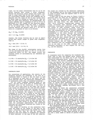
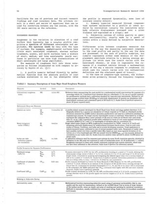
TABLE 3 Roughness Data by Various Measures in the International Road Roughness Experiment
Surface
Asphalt concrete
Surface treatment
Gravel
Earth
SEC
CAO!
CA02
CA03
CA04
CADS
CA06
CA07
CADS
CA09
CAIO
CAii
CA12
CA13
TSO!
TS02
TS03
TS04
TS05
TS06
TS07
TS08
TS09
TS!O
TSll
TS12
GROI
GR02
GR03
GR04
GROS
GR06
GR07
GROS
GR09
GRID
GR!!
GRJ2
TEO!
TE02
TE03
TE04
TE05
TE06
TE07
TEOB
TE09
TE!O
TEii
TEl2
!RI
4.1
4.6
6.3
5.3
6.2
7.3
2.5
2.6
3.S
3.3
S.4
1.9
1.9
4.3
5.I
4.7
5.5
5.7
3.3
3.3
4.0
3.9
3.8
2.S
2.5
3.7
3.8
7.2
6.4
9.2
8.3
s.s
4.4
9.2
7.1
14.1
12.7
4.3
4.1
7.2
7.3
13.9
16.6
4.4
s.o
8.6
10.2
9.6
9.0
IM,
260
291
399
336
393
463
!SS
165
222
209
342
120
120
272
323
298
348
361
209
209
2S3
247
241
158
!SS
234
241
456
406
S83
526
348
279
583
4SO
893
805
272
260
456
463
881
l,OS2
279
317
545
646
608
570
BI
1,970
2,340
3,690
3,280
4,220
5,02S
l,78S
1.775
2,420
2,235
3,S45
1,310
1,325
3,335
4,060
4,245
4,010
4,685
2,485
2,555
3,04S
3,150
3,33S
2,210
2,315
2,315
2,485
S,320
4,S65
6,985
7,010
3,970
2,910
6,060
4,65S
10,890
10,385
3,400
3,270
6,350
7,06S
13,3SO
16,48S
3,745
3,905
6,390
9,300
8,455
7,860
54
SS
75
66
78
96
33
34
51
4S
72
19
22
77
59
7S
IOI
124
37
38
46
43
44
28
27
36
38
90
77
133
117
80
54
105
94
187
180
53
51
90
94
164
211
65
67
94
121
111
99
QI,
47
61
84
75
87
95
29
?7
37
36
71
17
17
46
57
54
59
60
35
38
46
42
42
26
25
42
42
93
83
115
103
67
51
110
84
194
193
50
48
90
89
187
221
54
58
109
138
134
140
56 17.7 9.4
65 15.0 12.0
91 17.2 29.1
80 16.7 21.2
90 18.0 30.6
108 19.0 29.7
49 7.0 6.3
42 7.0 6.8
60 11.0 10.7
62 11.0 16.5
69 16.0 17.8
28 5.0 3.3
28 5.5 3.0
70 7.5 19.2
73 9.5 18.4
80 10.4 22.8
89 19.4 25.8
94 9.0 29.4
50 8.2 8.8
51 8.4 9.2
50 10.9 11.6
60 7.8 14.9
61 7.2 16.0
36 4.6 6.3
40 5.2 4.6
58 5.8 13.3
58 7.0 12.9
103 17.0 33.4
113 14.6 36.0
169 20.0 37.2
153 20.2 37.2
89 7.7 30.6
75 7.1 15.3
139 16.9 37.2
134 13.2 37.2
13.4
18.0
71 11.4 17.5
72 10.7 17.7
125 14.5 34.8
128 18.6 33.7
16.8
21.7
83 9.5 22.9
86 9.0 22.9
129 14.7 35 .0
156 17.3 37.2
158 16.8 37.2
108 18.1 37.1
122.2
80.4
119.3
141.5
159.6
78.9
28.5
17.4
33.l
45.5
136.3
11.2
10.5
18.4
39.8
27.4
25.0
20.8
27,3
39.0
61.5
18.0
20.7
13.6
7.8
17.4
14.2
94.6
109.9
104.1
117.8
42.4
16.9
98.6
94.6
51.7
35.4
93.7
181.9
43.8
30.4
107.2
155.I
155.0
148.0
Note: Refer to Table l for definition and units of roughness measurement.
Source: Derived from data given by Sayers et al. (6).
affected. A significnt difference does exist, how-
ever, between Qlr and Q1rn because of the non-zero
intercept in the definition of the Qir profit sta-
tistic (as will be seen in Table 4). Hence it was
important to use Qim instead of Qlr in this cor-
relation exercise.
The Bir data represent the roughness measured
by the Bump Integrator trailer at 32 km/h, which
were three-run averages of both wheelpaths. These
data represent the output of the trailer as it was
at the IRRE, under controlled operating conditions,
and were considered by TRRL to be representative of
its performance in previous studies.
The CP2.51 Wsw• Wmw• and CAPL25 numerics for the
APL profilometer were the section-mean values (across
both wheelpaths) of the values reported at the IRRE
[ (_~) , Appendix G] •
It can be seen that the data cover a wide range,
from very smooth (1.9 m/km IRI) to very rough (16.6
m/ km IRI) roads. Further conunent on the correlations
will be made later.
Analysis
The objective of the analysis was to develop practi-
cal conversion relationships among the various mea-
sures. Typically, when two variables are imperfectly
correlated, either both are measured with error or
the two represent different measures. In this situ-
ation, linear regressions of the one variable on the
other, and the o ther on t he one are nor mally not in-
terchangeable because the l east-squared deviations
differ in the t wo senses . For this analys i s , a con-
version relations hip was obtained by making l inear
least-squares estimates of coef ficien t s i n both
senses between each pair of variables and averaging
as follows:
Yi
The conversion equation should be such that
Y = p + qX and x = (Y - p)/q
take
p
q
(a - c/d)/2
(b + l/d)/2
(1)
(2)
(3)
(4)
(5)

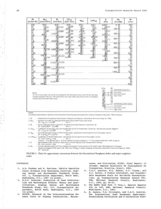
5. Paterson
where
Xit Yi
a,b,c,d
p, q
x, y
the ith pair of values of roughness
measures x and y, respectively;
residual errors of y and x, respec-
tively;
coefficients estimated by linear re-
gression;
coefficients adopted for conversion
equation; and
conversion equation estimates of x
y, respectively, given the other.
The goodness of fit of Equation 3 as a conversion
relationship was quantified by regressing the ob-
served values of Yi on the predicted values Yi
without intercept.
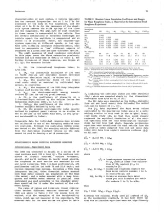
The resulting conversion relationships are given
in Table 4. The root mean squared error (RMSE) of
the conversion prediction and the estimated bias are
given for each. The bias in each case is very small,
typically less than 2 percent, and negligible.
A selection of the conversion relationships is
plotted with the observed data in Figures 1 and 2.
One observation is given per test section, and the
surfacing types are distinguished by symbols. Figure
1 shows the relationships between the Brazil Qim
scale, the TRRL BI scale, and the IR! scale, which
were pertinent to the major road costs studies. Fig-
ure 2 shows the relationships of three numerics of
the APL profilometer to the IR!.
53
Discussion of Relationships
Very high correlations exist between the IR! scale
and both the Qim and BI measures used in the major
empirical studies, so that interchange between either
of the historical measures and !RI can be made with
reasonable confidence. This is shown in Figures la
and le. The standard error: for estimating IRI rough-
ness was 0. 92 and O. 76 m/km IRI from Qim and BI
measures, respectively. From the plots it can be
seen that this error is reasonably uniform over the
range of roughness and across all four surface types.
A feature to note in the Qim data is that two
of the measurements on surface treatment pavements
are high values that appear as outliers in both Fig-
ures la and lb. The high values result not from a
shortcoming of the QI scale but from resonance of
the wheel-axle system in the specific vehicles used
for the Mays meters; th is occurred on two sections
that had minor surface corrugations at about 2 m
spacing. Neither profile statistic, IRI, or CP2.S•
was unduly affected by the corrugations, which re-
flects the good damping characteristics incorporated
in each one. The Bump Integrator trailer, traveling
at the slower speed of 32 km/ h compared with the 80
km/h speed of the Mays meter vehicle, was not af-
fected either, as shown in Figure le.
The BI trailer tends to be more sensitive to
earth roads than passenger cars (or IRI or Qim)
because of the particular characteristics of its
suspension system. The system has a resonant fre-
quency that corresponds to a wavelength of about
TABLE 4 Summary of Relationships and Statistics for Conversions Between
Roughness Scales
Conversion Relationship
E[!Rl) = Qlm/13
= (Ql, + 10)/14
= 0.0032 Bl 0
·
89
= CP2.s/I 6
"'5.5 log0 (5.0/PSI)
= 0.80 RARS.50
= 0.78 W,wo.oT
= CAPL25/3.0 if asphalt
_ = CAPL25/2.2 if not asphalt
E[Qiml = 13 !RI
= 9.5 + 0.90 Ql,
= jBl/55 if not earth
IBI/73 if earth
= 0.81 CP2.s
"' 72 Jog,, (5 .O/PSI)
= 7 9 w 0.70
• = 6:2 d.'PL2s
E[QI,] =-JO+I41RI
"'BI/62
=-I 0 + 0.89 CP2.s
E[BiJ = 630 IRJL 12
= 36 Qlml.12
= 155 Olm if not earth
73 Olm if earth
• = 62 QI,
E[CP2.s] = I6 IR!
= 11+1.12 QI,
= 1.23 Olm
= 1 J.7 w,wo.6s
(if CP2.s < 1SO)
No1e: !Hmihn... m l• codoo:
Standard
Error
0.919
0.442
0.764
0.654
0.478
0.693
1.050
12.0
14.5
11.7
11.7
8.78
18.29
6.32
14.0
13.l
694
1JOO
673
850
!0.5
14.8
14.4
8.87
Bl = TRRL Bum p lnfegr111tor lfftl er Df 31 km/h (mm/km).
Coefficient
of
Variation
15.4
7.34
12.7
12.4
15.3
18.7
15.0
17.2
8.35
18.3
20.3
14.7
22.8
14.2
18.1
12.4
17.6
17.2
CAP~s -= APJ.. proOlornetcr coofrichml for l. 1.6 km/h op~rnt i(Hl .
CP::i. s " AP.L prof'llome1er c0<rnclent of planarity (.0 I mm).
JR'! ~ lnltrnallon al llou&hn""' ~•d<• (m/km} ldono1cs RARSso (7/1.
Qlm ~ RTRRMS-ullmate of QI rou9hno55 in Oro>JI study (coun••/km).
QI, a l'rofilo RMSVA-functlon or QI rouahness (coun"/km).
Bias
Slope Units
0.989 m/km
0.975 m/km
1.008 m/km
0.993 m/km
m/km
1.002 m/km
0.994 m/km
1.030 m/km
0.993 Counts/km
0.985 Counts/km
1.002 Counts/km
0.986 Counts/km
Counts/km
0.996 Counts/km
1.13 Counts/km
1.024 Counts/km
1.006 Counts/km
0.980 Counts/km
0.998 mm/km
0.985 mm/km
0.976 mm/km
0.971 mm/km
0.994 0.01 mm
0.995 0.01 mm
0.986 0.01 mm
1.018 0.01 mm
llARSso ~ AllS rupon•• or refe r•nco rougllnl!S• sJmulatlon nl SO km/h (1}.
w,w =Shotl wa.vc:t<:ngrh (l h,1 3.3 nl) o.uargy h1de:x; V of APL.?2 prorilomiota.r a:s dc.rLucd by Frf:nCh LCP.C
I(6). Appondbc GI·
Source: Computer anmlyl.is.of da111 from tho l n ccir n ~Oomd Road Rough nc.u ExpcTlmt:n1 (6).

6. 54 Transportation Research Record 1084
(a)
~ (counl1/km)
210
180
150
+
120 x
90
'./'
Tl mTTIT1lnTTfTTITTTrT'1''"''"'fl m TTTTryTTTTTT~nrr.•rr
11 rr11rrrrrrrrrrrr
0 2 6 8 10 12 14 16
IRI (m/km)
(b)
Qlm (counts/km)
2101
180
150
120
90
60
.4°f'
':/ '
Qlm =0.81 CP2.s
+
""• '•"'l'''''''''l"'",,''l'"'""'l'""'Tf'l'"'"'"'"'f'"mTTrnt•••••••• 1
,,,
0 20 40 60 BO 100 120 140 160
CP2.s (001mm)
LEGEND:
lfGEND: • • • Asphalt Concrete x x x Eorth ROAD SURFACE: o • • Asphalt Concrete x x x Eorth
+
ROAD SURFACE: + + + Grovel tJ. l!. tJ. Surface Treatment + + + Grovel l!. tJ. l!. Surface Treatment
(c)
Blr(mm/km)
Bl,= 630 IR1112
+
x
...... jli Ojllllfiifi p I
0 2 6 8 10 12
IRl(m/km)
x
x
+
'I ""' I"~
14 16
(d)
Bl,(mm/km)
17.500
15.000
12.500
10.
5.0CO
2.500
0 20
LEGEND: LEGEND:
x
x
Bl,=55Qlm
40 60 80 100 120 140 160 180
Qlm (counts/km)
ROAD SURFACE: • o o Aspholt Concrete x x x Eorth ROAD SURFACE: o • o Asphalt Concrete x x x Earth
200
+ + + Grovel l!. tJ. l!. Surface Treatment + + + Grovel ll ll ll Surface Treatment
x
FIGURE l Relationships for conversion between Qlm (Brazil road costs study), BI (TRRL Bump Integrator trailer), and CP2.s (French/
Belgian APL profilometer) scales of road roughness: (a) Brazil calibrated Mays meter, Qlm, and profile roughness, IRI; (b) Brazil calibrated
Mays meter, Qlm, and APL72 profilometer coefficient, CP2.s; (c) TRRL Bump Integrator trailer at 32 km/h and profile roughness, IRI;
and (d) TRRL Bump Integrator trailer at 32 km/h and Brazil calibrated Mays meter, Qlm .
O. 76 m, and the shock absorbers are loosely damped
with gain levels 50 to 100 percent greater than typ-
ical passenger cars at the resonance frequencies.
Thus, the BI trailer responds to the strong short
wavelength content in earth surfaces with an exag-
gerated response, which results in the nonlinearity
evident in Figures le and ld for earth surfaces.
This also implies that high roughness measurements
coming from the BI trailer probably overstate the
response of a typical passenger car (even when
traveling at a comparably slow speed), so that the
nonlinearity is important when interpreting vehicle
operating cost relationships that are related to BI
trailer roughness.

7. . . ' . . ' . . .
Paterson
(a)
~5
35
30 cAPL25 = 3.0 IRI
(A!phalt Concrete)
SS
(b)
0 '•j~
i ;~o~
; .~~;j~il~
O~i1~·~·f~i
l'TTf'T'--r"T'TT"f'-t-t 'TftT1'~·r-r~·~
j ~~~~~
·~·i~j~i,._.
,I
0 2 4 6 8 10 12 14 16 0 2 4 6 8 10 12 14 16
Legend:
Rood Surface:
IRI (m/km)
1 • • Asphalt Concrete
+++Gravel
XXXEarth
A A A Surface Treatment
(c)
CP2.s
210
180
150
120
60
+
IRI (m/ km)
LEGEND:
ROAD SURFACE: I I I Asphalt Concrete
+++Gravel
CP2 5 = 16 IRI
+
+
x
+
;·x
•
xx x Earth
A A A Surface Treatment
T'fitfttt'n'ttt'11f'ITTn'fl '1"",-"""l'~'"1'"'"""'"T''"" 1 11 1
f 11111 1 1 1 1
i 1
IT
0 2 4 6 8 10 12 14 16
IRI (m/km)
LEGEND:
ROAD SURFACE: o o • Asphalt Concrete x x x Earth
+ + + Gravel A A A Surface Treatment
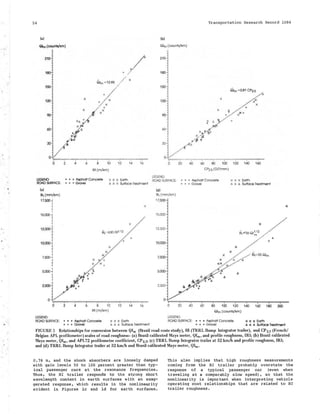
FIGURE 2 Relationships of various roughness coefficients of the French APL profilometer systems APL72 and APL25 to the
International Roughness Index: (a) APL25 profilometer coefficient, CAPL25, and profile roughness, IRI; (b) APL72 profilometer short
wavelength energy, W,w, and profile roughness, IRI: and (c) APL72 profilometer coefficient, CP2.s, and profile roughness, IRI.
On surfaces other than earth, the relationship
between the BI and Qim scales is virtually linear
as shown by the solid line in Figure ld. The rela-
tionship given as
BI (mm/km) = S5 Qim (counts/km) (6)
was derived in a separate analysis (9). Other stud-
ies have indicated that the value of the ratio (55)
can rise to 75 or higher when the BI trailer suspen-
sion system is not adequately maintained. Note that
when the measurement error is proportional to the
square root of the mean value [which is valid here,
see Paterson (_~)], and no intercept is expected be-
cause the measures are essentially similar (i.e.,
p = 0 in Equation 3), it can be shown that q in
Equation 3 is estimated by
(7)

8. 56
where-;;:, y are the mean values of x, y, respectively.
This result is particularly useful because it means
that a linear conversion under the foregoing condi-
tions can be derived simply from the ratio of the
mean values of each scale.
Of the various profile numerics developed for the
APL profilometer, the two that correlate the most
highly with vehicle response, and in particular the
IRI roughness scale, are the CP 2. 5 and short wave-
length energy (Wsw> indices shown in Figure 2 and
Table 2. The APL25 coefficient (CAP:Lis) has a yeu-
erally poor correlation with IRI and other response-
type measures because it is sensitive mostly to long
(7 to 15 m) rather than short wavelengths, and the
correlation is thus best on asphalt concrete sur-
faces (see Figure 2a and Table 4). All the APL sta-
tistics, except CPz .5, tend to reach signal satu-
ration as can be seen from Figures 2a and 2b. For
example, the Wsw index for the APL25 is not ap-
plicable to roughness levels above B m/km IRI. In
order to avoid mechanical damage, the APL profilom-
e ter was not operated on roaas with roughness greater
than 11 m/km IRI during the IRRE; that is, unpaved
roads with moderately high roughness.
RELATIONSHIP OF SERVICEABILITY INDEX TO ROUGHNESS
Roughness defined by a slope variance statistic was
included as one component of the Serviceability In-
SeNiceabillty
Index. SI (PSI)
5.0
4.5
4.0
3.5
3.0
2.5
2.0
1.5
1.0
0.5
Transportation Research Record 1084
dex function estimated from panel ratings of pave-
ment serviceability at the AASHO Road Test. Some at-
tempts have since been made to relate roughness to
serviceability by calibration of the vehicles to
slope variance and application of the original SI
function given in the AASHO Road Test (~). However,
it has been more common for agencies to relate rough-
ness directly to new local panel ratings of service-
ability (PSR) • Ratings, however, tend to vary con-
siderably with the expectation of the users and
U1.,iL vi:ev ious exposure to very high roughness
levels, so that the ratings typically vary from
country to country. SI was not defined for unpaved
roads,
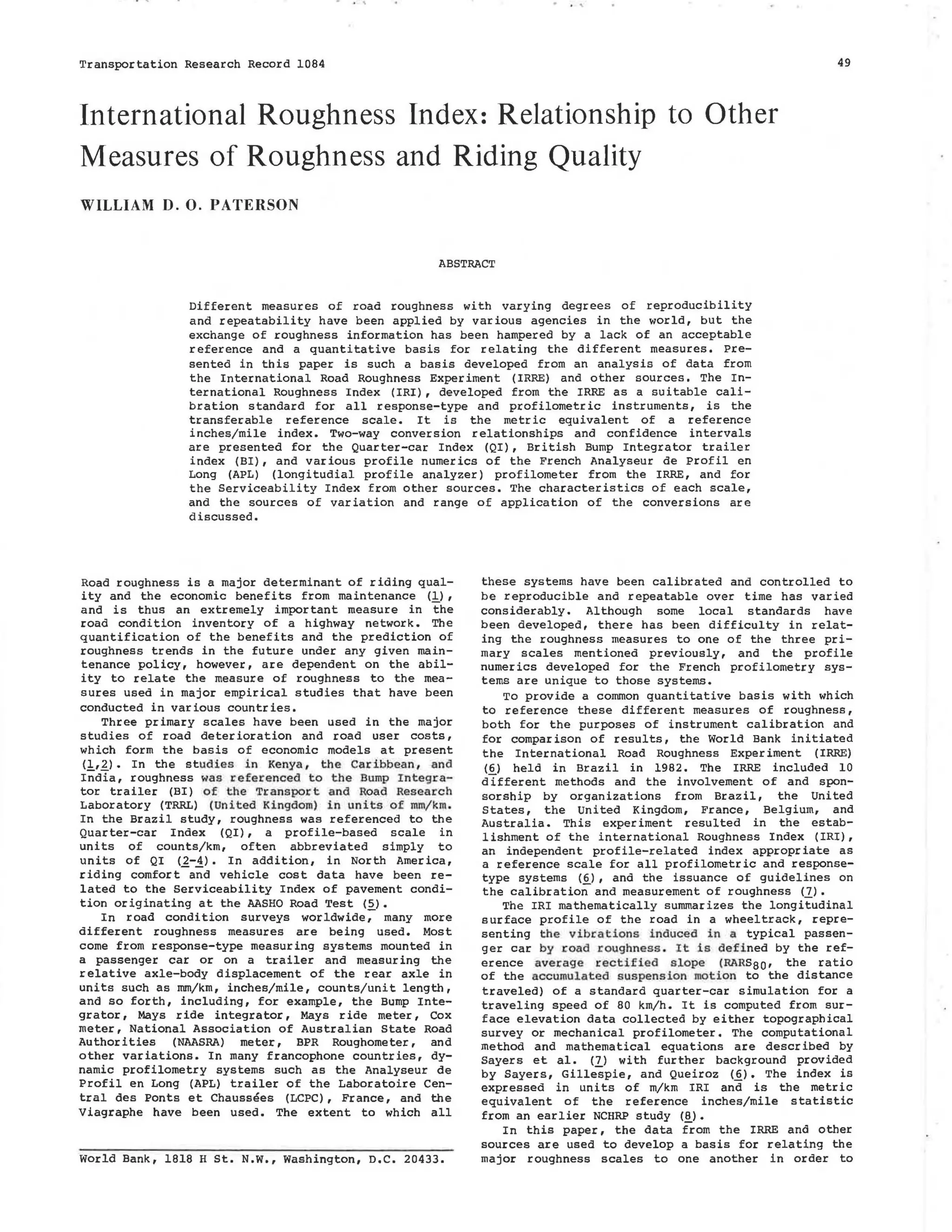
Relationships between PSR and the Qim and IRI
roughness scales are given in Figure 3. These were
derived from four panel rating sources: Brazil and
Texas [(l), Working Document 10] ,·south Africa (10),
and Pennsylvania (11). For the first three, PSR was
related directly t~he QI profile numeric; in Texas,
the panel rating was an estimate derived from a
waveband correlation with profile data derived in
Texas that was applied to Brazilian road profile
data. For the Pennsylvania relationship, an approxi-
mate conversion of 1 count/ km Qlro = 6.6 in./mi was
applied to the roughness data.
Considerable variations exist in the Serviceabil-
ity Index scales derived from the different sources:
the Texas, Pennsylvania, and South Africa ratings
represent users who are used to high-standard paved
~ s
0 4 8 12 16 20
Profile Roughness (m/km IRI)
I' ' I I I I I' I I I ' ' I I I I ' I I' I I I' I I I I I I I' I I I I I I I'' I I I I Ii I I
0 W 100 1W 200 200
Legend:
Roughness Qlm(Counts/km)
X - - - Texas
N - - - NCHRP228
p -----· PennDOT
B - - Brazil
S - - - - South Africa
T - TRDF
FIGURE 3 Approximate relationships between AASHO serviceability
index, PSI, and the Qlm and IRI roughness scales, based on panel ratings
from four sources.

9. Paterson
roads, but the means nevertheless vary by up to one
rating interval when rating a given roughness,
whereas the Brazilian raters attach much higher rat-
ings to rough roads than do the other groups. A lin-
ear relationship between rating and roughness may be
adequate over the range of two to four rating units
on paved roads as claimed by Janoff et al. (12) but
does not apply more generally. By extrapolation, the
scales indicate that a roughness of 130 to 175 QI is
equivalent to O PSI, except for the Brazilian panel,
which included unpaved roads and rated a roughness
of 175 as better than 1 PSI. The best continuous
function meeting the perfect score of 5 on the SI
scale at a roughness of zero is as follows:
Q1m 72 loge (5. O/SI)
IRI 5.5 loge (5.0/SI)
However, the linear function may be just as appro-
priate over normal ranges of paved road roughness,
that is
Q1m max [136 - 33 Sii OJ
IRI max [10.5 - 2.5 Sii OJ
The slope of the Qim/PSI relationship varies from
-20 for serviceability above 3.5 PSI to -33 for ser-
viceability below 3. 0 PSI. The common initial and
terminal levels of serviceability are therefore ap-
proximately
4. 2 PSI 13 counts/km Qlm 1.0 k/km IRI
2.5 PSI 50 counts/km Qim 3.8 m/km IR!
2.0 PSI 65 counts/km Qim 5.0 m/km IRI
1. 5 PSI 86 counts/km Qim 6.6 m/km !RI
CONVERSION CHART
For convenience of application, the results of the
foregoing analyses are presented in the form of a
conversion chart in Figure 4. The IRI scale is used
as a reference on each side of the chart, and for
North American users, the equivalent reference scale
in inches/mile units (IMrl is presented alongside.
For all other roughness measures shown on the
chart, the bars have three sets of graduations, the
estimated value on the centerline, a low value on
the left, and a high value on the right. The low and
high values are defined by the 15th and 85th percen-
tiles of the preceding data and indicate the range
over which the actual value for a specific road sec-
tion can be expected. For example, to estimate the
roughness of 6 m/km IRI in terms of the Qim scale,
an estimated value of 78 counts/km Qlm is obtained,
and the authors are about 70 percent confident that
the actual value will be between 66 and 90. For con-
verting between two of the nonreference scales, the
centerline of the given scale is used, and the esti-
mated low and high values of the desired scale are
read. For calculator applications, the conversion
functions and confidence intervals are listed at the
bottom of the chart.
The ranges of validity of the conversion func-
tions are shown by the length of the bars on the
chart. Individual observations may exceed the ranges
shown on the IRI, Qim, BI, and IMr scales, but
typically such high levels of roughness are confined
to short sections. In the case of the APL numerics,
57
the ranges are limited by the mechanical capability
of the equipment and by the signal processing method
to cases of paved roads and unpaved roads of low to
moderate roughness.
A chart such as the one shown in Figure 4 meets a
practical need, but there are two important caveats.
First there is the potential inference that the
various roughness measures are interchangeable and
measure the same thing. The IRRE showed clearly
that, while different response-type systems were
highly correlated when operated under identical
conditions, significant variations do exist between
the scales on some surfaces. These arise from
differences in the operating conditions, equipment,
wear, and interpretation of the diverse spectrum of
wavelengths in a road profile. These variations are
accommodated in the chart through the confidence
intervals, which indicate that the conversions are
approximate and give the range within which the
actual value may vary. Second, there is no guarantee
that the data collected at the IRRE are exactly
representative of the historical data collected in
previous studies. Not all these studies will have
been conducted with the recommended degree of con-
trol as was done at the IRRE, although there is
reasonable confidence in this respect for the Qim,
Bir, and APL measures.
CONCLUSION
An acceptable basis for comparing the roughness mea-
sures used in past and present major studies has
been established for use where one of the following
calibration references exist: BirQim, CP2.s• IMr or
IRI. However, the various roughness measures sense,
filter, and amplify the road profile characteristics
in different ways so that exact equivalences do not
exist between them. The conversion chart and rela-
tionships, shown in Figure 4, present the means for
comparing a number of scales that have been in use
and for relating them to the International Roughness
Index. These conversions and their inexactness were
based primarily on data from the international ex-
periment conducted in Brazil, and they are generally
valid only over the range of asphalt, surface treat-
ment, gravel, and earth surface types included in
the experiment. That validity, however, covers a
wide range, and significant deviations are only
likely on extremely different surface types, includ-
ing surfaces with periodic defects, such as corruga-
tions, or strong short wavelength content such as
potholed roads, earth roads, surfaces placed by man-
ual labor (macadams, cobbles, set-stones, etc.), and
coarse-gravel roads.
The degree to which the conversions presented
here are applicable to either historical or present
measurements made with a system similar to one of
those described, depends largely on how the operat-
ing conditions compare with those existing at the
IRRE. In the case of the profile-related systems
(Q1m, Wsw• and CP2.5), which are time-stable, the de-
gree of confidence is high. In the case of the Bump
Integrator trailer, and other systems using hardware
as a reference, the applicability depends on the de-
gree of similarity of the hardware to the system
used at the IRRE, which can differ in extreme cases
by up to 40 percent when out of calibration.
The widespread adoption of IRI as a reference and
calibration standard is being encouraged worldwide
to improve the reliability of exchanging information
related to road roughness. The IRI would then be a
common denominator, in some cases existing in paral-
lel with a local index or series of profile statis-
tics.

10. .·
58 Transportation Research Record 1084
IRI I Qlm I Bir I CP25 I Wsw
I CAPL25
I
SI IMr
I
IRI
(m/km IRI) (count/km) (mm/km) (0.01 mm) (PSI) (in/mile) m/km
0 0 0 0 0 0 5.0 0 0
, 20 ,, 1.000 20 40
2 20 1;'4 4 4.0 1
100- 2
, 40 ,... 2.000 , 40 4v v a 4
I 8
130
40 1 2.000 40 , 60 all v12 200-
4 I 3.0 1 20 4
1/4.uuu 60 , ao 12 20 8 12 I
)
II 300-
~ 80 4.0001 , 80 ) 100 16 2.0 I I
15
6 2QV 28 6
''i/ 6.000 11 36
400- -
80' 1 ~ 120 12 1.0
100 J 28 II 20
8 I 500 .~
120 140 ts
6.00011 '/ 8.000
120
II 160 16 0.5
10 140 I 36 I 600-- 10
120 160 8,000 I/10,000 160 II 1.0
20 700-
12
0.5
12
16011/
10,000 I/ 12.000 800-
14 14
200
12.000
1 14.000 900- --
16 1.000 16
-
200 240 14,000 16,000
18 18
16,000
20 ~40 20
Other IRI
ESTIMATING IRI SCALE
Notes: Low value
I Estimated value
On the 3-line scales. the center line represents the estimated value. and the left and right
High Value
margins represent the low (15th percentile) and high (85th percentile) limits of individual
values about the estimated value J
v
J
v ESTIMATING OTHER SCALE
• Low Value
Estimated value
~value
NOTES.
Conversions estimated on data from the International Rood Roughness Experiment. (Sayers, Gillespie and Queiroz. 1986) as follows
1 IRI - International Roughness Index (Sayers. Gillespie and Paterson. World Bank Technical Poper 46. 1986)
2. Qlm - Quarter-car Index of calibrated Moysmeter. Brozil-UNDP Rood Costs Study
IRI = Qlm/13 ± 0.37/iRf IR1<17
3 Bl, - Bump Integrator trrnler at 32 km/h. Transport and Rood Research Laboratory, UK
1ii1 =0.0032 B10,a9 ±0.31.lfRi; IR1<17
4 CP2 5 - Coefficient of planarity over 2 5m boselength for APL72 Profilometer. Centre de Recherches Rout1ers. Belgium:
IRI = CP2sf16 ±0.27/iR[ IRl<11
5. W5W - Short Wavelength Energy for APL72 Profilometer. Laborotoire Central des Pants et Choussees. France
IRI =0.78 w..,,D.63 ±0.69 IRI. IRl<9
6. CAPL25 - <;;oettident of APL25 Profilameter. Laboratoire Central des Pants et Choussees. Fronce
IRI =0,45 k CAPL25 ± 16%; IRI<11
where k = 1 for general use, k =O 74 for asphalt concrete surfaces. k =1 11 for surface treatment. earth or gravel.
7 SI - Serviceability Index. American Association of State Highway and Transportation Officials:
IRI =5.5 In (5.0/SI) ±25%: IRl<12
8. IM, - Inches/mile equivalent of IRI from Reference Quarter-Car Simulation at 50 mile/hr (see 'HSRl-reference· in Gillespie,
Sayers and Segel NCHRP report 228. 1980: and 'RARSao' in Sayers, Gillespie and Queiroz, World Bank Technical Paper 45. 1986):
IRI = IM,/63 36
FIGURE 4 Chart for approximate conversiom between the International Roughness Index and major roughness
scales.
REFERENCES nance, and Utilization (PICR). Final Report, 12
volumes. Empresa Brasileira de Planejamento de
Transportes, Brasilia, Brazil, 1982.
1 . A.D. Chesher and R. Harrison. Vehicle Operating
Costs: Evidence From Developing Countries. High-
way Design and Maintenance Standards Study,
Vol. 1, Transportation Department, World Bank,
Washington, D.c., 1987 (in press).
2. W.D.O. Paterson. Prediction of Road Deteriora-
tion and Maintenance Effects: Theory and Quan-
tification. Highway Design and Maintenance
Standards Study, Vol. III. Transportation De-
partment, World Bank, Washington, D.C., 1987
(in press).
3. GEIPOT. Research on the Interrelationships Be-
tween Costs of Highway Construction, Mainte-
4. C.A.V. Queiroz, W.R. Hudson, A.T. Visser, and
B.C. Butler. A Stable Consistent, and Transfer-
able Roughness Scale for Worldwide Standardiza-
tion. In Transportation Research Record 997,
TRB, National Research Council, Washington,
D.C., 1984, pp. 46-55.
5. The AASHO Road Test (7 Vols.). Special Reports
61A to 61G. HRB, National Research Council,
Washington, D.C., 1962.
6. M. Sayers, T.D. Gillespie, and C.A.V. Queiroz.
The International Road Roughness Experiment:
Establishing Correlation and a Calibration Stan-