In Korea's road design criteria, the guideline to evaluate the safety of horizontal curve and vertical curve is quantitatively suggested, but for a complex alignment where these two alignments are combined, qualitative guideline only is provided. Thus, the measure to quantitatively evaluate the safety of the complex alignment needs to be provided as early as possible. The useful approaches to the study introduced to date include the method to use running speed profile, the method to use the sight distance and the method to use the work load and the method to evaluate the safety of road alignment using running speed profile has been more widely applied than others. Many studies on evaluating the safety of road alignment using running speed profile have been conducted domestically which however are limited to the prediction model for running speed on horizontal alignment and the study on model to predict the complex alignment combining the horizontal alignment with vertical alignment has still been far behind. This study is intended to review the method using running speed profile among the methods to evaluate the safety of complex alignment and before developing the running speed prediction model considering the effect of complex alignment, the study was conducted as part of the review of the need for developing the model which is differentiated by the type of combination of horizontal alignment and vertical alignment. As part of the process, integrated running speed prediction model using the design elements of horizontal alignment as independent variable was developed which was then classified depending on combination pattern of horizontal alignment and vertical alignment and was compared with determination coefficient of prediction model for individual running speed. As a result, prediction model for individual running speed developed depending on combination pattern of horizontal alignment and vertical alignment was able to predict the running speed more accurately than integrated running speed prediction model, which implies the need for developing the running speed prediction model including the variables that incorporate the combination characteristics of unique horizontal alignment and vertical alignment.

1. International Journal of Engineering Science Invention
ISSN (Online): 2319 – 6734, ISSN (Print): 2319 – 6726
www.ijesi.org ||Volume 5 Issue 12|| December 2016 || PP.34-42
www.ijesi.org 34 | Page
Review of Applicability of Prediction Model for Running Speed
on Horizontal Curve
1
Wonbum Cho, 2
Chunjoo Yoon
1,2
Senior Researcher, Korea Institute of Civil Engineering and Building Technology, Korea
ABSTRACT: In Korea's road design criteria, the guideline to evaluate the safety of horizontal curve and
vertical curve is quantitatively suggested, but for a complex alignment where these two alignments are
combined, qualitative guideline only is provided. Thus, the measure to quantitatively evaluate the safety of the
complex alignment needs to be provided as early as possible. The useful approaches to the study introduced to
date include the method to use running speed profile, the method to use the sight distance and the method to use
the work load and the method to evaluate the safety of road alignment using running speed profile has been
more widely applied than others. Many studies on evaluating the safety of road alignment using running speed
profile have been conducted domestically which however are limited to the prediction model for running speed
on horizontal alignment and the study on model to predict the complex alignment combining the horizontal
alignment with vertical alignment has still been far behind. This study is intended to review the method using
running speed profile among the methods to evaluate the safety of complex alignment and before developing the
running speed prediction model considering the effect of complex alignment, the study was conducted as part of
the review of the need for developing the model which is differentiated by the type of combination of horizontal
alignment and vertical alignment. As part of the process, integrated running speed prediction model using the
design elements of horizontal alignment as independent variable was developed which was then classified
depending on combination pattern of horizontal alignment and vertical alignment and was compared with
determination coefficient of prediction model for individual running speed. As a result, prediction model for
individual running speed developed depending on combination pattern of horizontal alignment and vertical
alignment was able to predict the running speed more accurately than integrated running speed prediction
model, which implies the need for developing the running speed prediction model including the variables that
incorporate the combination characteristics of unique horizontal alignment and vertical alignment.
Keywords:road design, horizontal alignment, vertical alignment, alignment safety, running speed
I. INTRODUCTION
1.1. Background and Objective of Study
Traffic accident on road is caused by combination of three elements including driver, vehicle and road.
28% of the traffic accident was found to have been influenced directly or indirectly by road environment
(geometric structure of the road, weather) which is equivalent to ￦4.6trillion of annual loss totaled ￦15.0
trillion for traffic accident.
As part of the study for evaluating the safety of geometric structure among road environment,
development of running speed prediction model considering the geometric structure and evaluation of design
consistency using running speed are underway recently. Such running speed prediction model is mostly based
on design elements elating to horizontal alignment and the study on model to predict the complex alignment
combining the horizontal alignment with vertical alignment has still been far behind.
This study thus is intended to develop the running speed prediction model which incorporates the
design elements of horizontal alignment only using the speed data from the site and then review the possibility
of evaluating the design consistency of the complex alignment where horizontal alignment and vertical
alignment are combined.
1.2. Scope of the study and method
This study, within a spatial range of a 4-lane rural road where horizontal alignment and vertical
alignment are combined and within a time range of non-peak hour when the interference among the vehicles has
less effect on running speed, is aimed at investigating the driver's running speed.
A running speed prediction model that incorporates the design elements of horizontal alignment only
was developed using the speed data collected from the site and furthermore, a running speed prediction model
incorporating each influential factor by type classified as Table 1 and Fig. 1 depending on combination of
horizontal alignment and vertical alignment. Each running speed prediction model was compared each other
using determination coefficient and then the review whether a running speed prediction model incorporating the

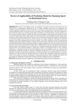
2. Review of Applicability of Prediction Model for Running Speed on Horizontal Curve
www.ijesi.org 35 | Page
design elements of horizontal alignment only is able to predict the running speed on vertical alignment The type
A in Table 1 and Fig. 1 is the case when the horizontal curve is on a flatland (hereinafter "horizontal alignment
section") and type B is the case when horizontal curve is on upward or downward alignment where a certain
vertical slope is maintained (hereinafter "vertical slope section") and type C is the case when horizontal curve is
on concave or convex vertical curve (hereinafter "complex alignment section")
Table 1. Classification depending on combination of horizontal alignment and vertical alignment
Fig. 1. Classification depending on combination of horizontal alignment and vertical alignment
II. BIBLIOGRAPHIC SEARCH
2.1 Running speed prediction model on horizontal alignment
Lamm et al (1995) proposed the model in Equation (2) below in the study on 85% of running speed and
horizontal curve.
V85 = 93.87 – 3171/R, R2
= 0.787 (2)
where, V85 : 85% of running speed (km/h)
R :horizontal curve radius (m)
R2
: coefficient of determination
Kanellaidis et al (1990) proposed the relational expression between horizontal curve and running speed as
follows.
V85 = 129.88 – 623.1/ ,R2
= 0.78 (3)
where, V85 : 85% of running speed (km/h)
R :horizontal curve radius (m)
R2
: coefficient of determination
Krammes et al (1994) proposed regression model with horizontal curve radius, angle of intersection and
superelevation as independent variables.
V85 = 102.45 – 2741/R + 0.0037-0.10Θ,R2
= 0.82 (4)
where, V85 : 85% of running speed (km/h)
R :horizontal curve radius (m)
R2
: coefficient of determination
L :horizontal curve length (m)
Θ : angle of intersection (˚)
Type Vertical alignment Horizontal alignment
A flatland Horizontal curve
B B1 upward slope
B2 downward slope
C C1 concave vertical curve
C2 convex vertical curve

3. Review of Applicability of Prediction Model for Running Speed on Horizontal Curve
www.ijesi.org 36 | Page
2.2 Running speed profile model on complex alignment
Fitzpatrick et al (2000) classified it into 10 categories depending on combination of horizontal alignment and
vertical alignment and proposed running speed prediction model as Table 2.
Table 2. Running speed prediction formula by alignment condition
No Alignment conditions Speed prediction formula
1 Horizontal curve-Vertical slope
-9% ≤ G 〈 -4%
V85=102.10- 3077.13/R
2 Horizontal curve-Vertical slope
-4% ≤ G 〈 0%
V85=105.98 – 3709.9/R
3 Horizontal curve-Vertical slope
0% ≤ G 〈4%
V85=104.82 – 3574.51/R
4 Horizontal curve-Vertical slope
4% ≤ G 〈 9%
V85=96.61 – 2752.19/R
5 Horizontal curve-Concave vertical curve V85=105.32 – 3498.19/R
6 Horizontal curve-Convex vertical curve
(no sight distance limit)
Min speed predicted in equation 1, 2
(downward) and 3 & 4(upward)
7 Horizontal curve-Convex vertical curve
(sight distance limit)
V85=103.24 – 3576.51/R
8 Horizontal straight-Concave vertical curve V85=assumed desired speed
9 Horizontal straight-Convex vertical curve
(no sight distance limit)
V85=assumed desired speed
10 Horizontal straight-Convex vertical curve
(sight distance limit)
V85=105.08 – 149.69/K
III. DATA COLLECTION AND ANALYSIS
In this study, monitoring of running speed was conducted at 66 points on national highway #5, 6, 42
and 44 as part of the effort to develop the running speed prediction model. The roads where the monitoring was
conducted were high standard road where horizontal alignment and vertical alignment are distributed diversely
and the data on geometric structure and driver's running speed was collected.
3.1 Selection of the points
In this study, the points which meet the principle for selection were chosen in a bid to develop the running speed
prediction model that incorporates the effect by horizontal alignment and vertical alignment.
• Where no effect of intersection
• Where no effect of overspeed control system
• Where the effect by surrounding environment is minimized
• Where no school, bridge or factory that may cause abnormal situation to the driver
After surveying the candidate sites referring to the road drawing, the sites were selected finally and the
distribution of the sites is as Table 3 But in type A, flatland was determined based on vertical slope ±2% or less.
Table 3. Distribution of the sites by type
Type Vertical alignment No Total
A Flatland 23 23
B B1 Up hill 10 19
B B2 Down hill 9 19
C C1 Convex vertical curve 13 24
C C2 Concave vertical curve 11 24
Total 66
3.2. Geometric structure of the road
The elements of road geometric structure were collected from road design document. The data
collected were horizontal curve radius (R), horizontal curve length (CL), superelevation (e), lane width (LW),
shoulder width (SW), vertical slope (G), algebraic difference of vertical slope (A), vertical curve length (Lv),
distance between inflection points of horizontal curve and vertical curve (Lo) and variation rate of vertical curve
(K)
Table 4 shows minimum and maximum range of road geometric structure depending on combination of
horizontal and vertical alignment. Horizontal curve radius (R) is distributed over 300～3,000m while vertical

4. Review of Applicability of Prediction Model for Running Speed on Horizontal Curve
www.ijesi.org 37 | Page
alignment (G) is -5.9～4.8%. Vertical slope difference (A) in Type C, a complex alignment is 0.7～6.3% and
vertical slope variation rate (K) is 17.1～290.7.
Table 4. Geometric structure by type
Geometric element Complex alignment type
Type A Type B Type C
R(m) 300～1,000 300～2,000 300～3,000
CL(m) 114～987 105～626 128～693
e(%) 2.0～6.5 1.5～6.9 2.0～6.0
LW(m) 3.4～3.6 3.4～3.6 3.4～3.6
SW(m) 1.3～2.0 1.0～2.5 1.5～2.3
G(%) -1.5～1.6 -5.9～4.8 -3.8～3.6
Lv(m) - - 70～1,140
A(%) - - 0.7～6.3
L0(m) - - 1～194
K(m) - - 17.1～290.7
3.3. Monitoring of running speed
Data on speed was collected using American nu-metrics' NC-97. The detector was 16cm wide, 14cm
long and 2cm high which is not easily identified by the driver. The detector detects the vehicle passing above
the magnetic field and the microcomputer in detector predicts the spot speed. The data from the detector
includes vehicle speed, detection time, headway and vehicle length which are stored at the detector and then
transferred to PC through RS232 port after investigation.
The data was collected at 100m ahead of the curve and in middle of the curve (hereinafter '1/2L') and
additional detector was set at the point where sight distance is limited when vertical alignment in complex
alignment section (type C) is in convex shape (hereinafter "convex curve") and at the peak on concave curve
when vertical alignment is in concave shape (hereinafter "concave curve")
Fig. 2.shows the location of detector by type of road alignment.
Fig.2. Location of detector by type of road alignment
In case of headway 6 seconds or less, it's excluded from the data on assumption of being influenced by other
vehicles and passenger car only was included for analysis.
3.4. Development of running speed prediction model
This study is intended to determine the possibility of evaluating the design consistencyin the section
where horizontal alignment and vertical alignment are combined through running speed prediction model that
considers horizontal alignment design element alone and thus a running speed prediction model including both
horizontal alignment, vertical alignment and combined curve alignment (hereinafter called ‘Integrated model’)
and a running speed prediction model depending on type of combination of horizontal alignment and vertical
alignment (hereinafter called ‘Individual model’) are developed, separately.
Detector 1: Type A,B,C: 100m ahead of horizontal curve
Detector 2: Type A,B,C:1/2L of horizontal curve
Detector 3: Type C (convex): where sight distance is limited
Type C (concave):correction of concave horizontal curve

5. Review of Applicability of Prediction Model for Running Speed on Horizontal Curve
www.ijesi.org 38 | Page
Table 5 shows the classification by the type of combination of horizontal alignment and vertical
alignment and suggests the representative type of running speed prediction model.
'Type A' is the section where horizontal curve and flatland are overlapped and as suggested by previous
studies, design element of horizontal alignment (R') is the key parameter in predicting the running speed (see 1)
of Table 5) 'Type B' is the horizontal curve where a certain slope is maintained and prediction model containing
the design element of horizontal alignment (R') and design element of vertical slope (G') as independent variable
would be important (see 2) of Table 5) 'Type C' is the case combining horizontal alignment and vertical
alignment and prediction model containing design element of horizontal alignment (R') and design element
relating to vertical slope (K') may be assumed (see 3)～5) of Table 5).
Table 5. Running speed prediction model by type of road alignment
Type Prediction model
A 1) V85=bo+b1×R'
B 2) V85=bo+b1×R'+b2×G'
C 3) V85=bo+b1×K'
4) V85=bo+b1×R'+b2×K'
5) V85=bo+b1×(R'×K')
where, R'
G'
K'
:
:
:
design element of horizontal alignment
design element of vertical slope
design element of vertical curve
Based on prediction model proposed in Table 5, integrated model with V85 as dependent variable and
with design element of horizontal alignment as independent variable and individual model with design element
of each type of road alignment as independent variable were developed. In this process, the lower value speed
data among those from detector 2 and 3 was used.
In addition to common variables, square and square root of each variable, natural logarithms and
exponential function were also reviewed for developing the prediction model.
The variables considered to predict the running speed are as Table 6.
Table6. Independent variables
Design elements of horizontal alignment (R')
․1/R : Curvature (m-1)
․CL : Horizontal curve length (m)
․LW : Lane width on horizontal curve (m)
․SW : Shoulder width on horizontal curve (m)
․e : Superelevation on horizontal curve (%)
Others : Square, square root, natural logarithms and exponential function by design element of
horizontal alignment
Design elements of vertical alignment (G', K')
․G : Vertical slope (%)
․A : Algebraic difference of vertical slope (%)
․Lo : Distance between infection points of vertical curve and horizontal curve (m)
․Lv : Vertical curve length (m)
․K : Variation rate of vertical curve (m/%)
Others : Square, square root, natural logarithms and exponential function by design element of
vertical alignment
Independent variable of regression model was selected considering the significant design element with
higher correlation with V85 and the primary regression model was developed in a way of eliminating one by
one the independent variable failed to meet the elimination requirement (F=0.010) Optimal regression model
was determined among the primary regression models considering the sign of independent variable, correlation
between independent variables, significance of model and independent variable (F testing hypothesis, t testing
hypothesis) independence between error terms (Durbin-Watson), multicollinearity (tolerance limit VIF, state
index), outlier (standardized residuals).
When it comes to determination coefficient indicating the explanation power of regression equation,
modified determination coefficient (adj R2
) was applied to minimize the effect of increasing determination
coefficient by increase in number of independent variables.
1) Integrated model
A running speed prediction model that incorporates horizontal design elements from 66 survey points
was developed. Table 7.summarize the optimal integrated regression model and the reg4ression model with 1/R
and e as independent variable was found to be most persuadable. As a result of F, t test, determined regression
model and individual independent variable have statistical significance and regression model determined by

6. Review of Applicability of Prediction Model for Running Speed on Horizontal Curve
www.ijesi.org 39 | Page
residual and multicollinearity analysis was found not to be in conflict with basic assumption of regression
model. A determination coefficient of optimal regression model was 0.134.
Table7. Integrated optimal regression model
Model Non-standardized coefficient t Significanceprobability Colinearity statistic R2
B Standard error Tolerance limit VIF
Constant 106.19 2.294 42.285 .000 .134
1/R -7229.22 2085.702 -3.466 .001 .246 4.060
e 3.14 1.070 2.933 .005 .246 4.060
V85=106.19 - 7229.22×1/ +3.14×e
where, V85
R
e
:
:
:
85 percentile running speed (km/h)
horizontal curve radius (m)
superelevation(%)
2) Individual model
(1) ‘Type A’
A ‘Type A’ running speed prediction model was developed using V85 data from 23points and
horizontal alignment design element. Table 8 summarizes ‘Type A’ optimal regression model. According to
analysis, regression model with 1/ and e2
as independent variable was most persuadable and determination
coefficient of regression model was 0.256.
Table 8.‘Type A’ optimal regression model 1
Model Non-standardized
coefficient
t Significance
probability
Colinearity
statistic
R2
B Standard error Tolerance
limit
VIF
Constant 124.89 7.922 15.627 .000 .256
1/ -634.55 229.826 -2.761 .012 .420 2.378
e2
0.46 0.152 3.006 .007 .420 2.378
V85=124.89 - 634.55×1/ +0.46×e2
where, V85
R
e
:
:
:
85 percentile running speed (km/h)
horizontal curve radius (m)
superelevation(%)
Regression model with 1/R which was proposed in previous studies as independent variable is as Table 9.
Table 9.‘Type A’ optimal regression model 2
Model Non-standardized
coefficient
t Significance
probability
Colinearity
statistic
R2
B Standard
error
Tolerance
limit
VIF
Constant 110.76 3.697 29.957 .000 .208
1/R -6553.45 2684.085 -2.442 .024 .443 2.258
e 0.42 .153 2.722 .013 .443 2.258
V85=110.76 - 6553.45×1/ +0.42×e
where, V85
R
e
:
:
:
85 percentile running speed (km/h)
horizontal curve radius (m)
superelevation(%)
As a result of F, t test, determined regression model and individual independent variable have statistical
significance and regression model determined by residual and multicollinearity analysis was found not to be in
conflict with basic assumption of regression model.
Individual model developed from Type A has higher determination coefficient than integrated model, indicating
enhanced running speed prediction performance.
(2) ‘Type A’ + ‘Type B’
‘Type B’running speed prediction model was planned to be developed using V85 data from 19 points
and design elements with regard to horizontal alignment and vertical slope, but because of nor available of
significant regression equation, a running speed prediction model was developed with total 42 points in a way of
combining ‘Type A’ and ‘Type B’. Table 10 summarizes the running speed prediction model considering the
integration of ‘Type A’and‘Type B’. Similarly with Type A running speed prediction model, regression model

7. Review of Applicability of Prediction Model for Running Speed on Horizontal Curve
www.ijesi.org 40 | Page
with 1/ and was independent variable was most persuadable. Determination coefficient of regression equation
was 0.179, indicating lower running speed prediction performance than ‘Type A’ running speed prediction
model. .
Table 10. ‘Type A’+‘TypeB’ optimal regression model
Model Non-standardized
coefficient
t Significance
probability
Colinearity statistic R2
B Standard
error
Tolerance
limit
VIF
Constant 118.47 4.718 25.107 .000 .1
791/ -618.19 188.215 -3.285 .002 .246 4.058
e 3.37 1.102 3.062 .004 .246 4.058
V85=118.47 - 618.19×1/ +3.37×e
where, V85
R
e
:
:
:
85 percentile running speed (km/h)
horizontal curve radius (m)
superelevation (%)
(3) ‘Type C’
A ‘Type C’ vertical curve running speed prediction model was developed using horizontal convex curve from
13 points and V85 data from horizontal concave curve from 11 points and vertical curve design elements
① ‘Horizontal convex curve’
Table 11summarizes the optimal regression model of horizontal convex curve. As a result of regression
analysis based on independent variables which were not excluded by removal standard, regression model with
Lo and exp(e) that incorporate the relationship between horizontal curve and vertical curve as independent
variables was most persuadable. Determination coefficient was 0.475 and running speed prediction performance
was enhanced when comparing with determination coefficient of integrated model, 0.134.
Table 11. Optimal regression model of horizontal convex curve
Model Non-standardized
coefficient
t Significance
probability
Colinearity statistic R2
B Standard
error
Tolerance
limit
VIF
Constant 112.07 2.601 43.096 .000 .475
Lo -0.047 0.081 -2.616 .024 1.000 1.000
exp(e) -0.058 0.024 -2.408 .037 1.000 1.000
V85=112.07 - 0.047×Lo-0.058×exp(e)
Where, V85
Lo
e
:
:
:
85 percentile running speed (km/h)
distance between inflection points of vertical curve and horizontal curve(m)
superelevation(%)
Table 12 shows the result after removing independent variable one by one from optimal regression
model. Lowhich is determined by correlation between horizontal alignment and vertical alignment design
element was found to have larger effect on running speed prediction performance than e which is horizontal
alignment design element. Such result shows that a running speed prediction model incorporating the effect by
linear combination needs to be considered for the alignment where horizontal curve and vertical curve are
combined.
Table 12. Regression model considering the effect of Loor e
Model Independent
variable
Regression model R2
1 Lo V85=107.22 - 0.048×Lo .240
2 exp(e) V85=108.97 - 0.058×exp(e) .188
Where, V85
Lo
e
:
:
:
85 percentile running speed (km/h)
distance between inflection points of vertical curve and
horizontal curve(m)
superelevation %)
②‘Horizontal convex curve + horizontal concave curve’

8. Review of Applicability of Prediction Model for Running Speed on Horizontal Curve
www.ijesi.org 41 | Page
A running speed prediction model for horizontal concave curve was planned to be developed using
V85 data from 11 points and horizontal alignment and vertical curve design elements but significant regression
equation was not available and thus a running speed prediction model was developed with total 24 points in a
way of combining horizontal convex curve and horizontal concave curve. Table 13 summarizes the running
speed prediction model that is applicable to both horizontal convex curve and horizontal concave curve.
Regression model with Lo and1/Ln(R) as independent variable was most persuadable. Determination coefficient
of regression equation was 0.251, indicating a lower determination coefficient comparing to the running speed
prediction model for horizontal convex curve.
Table 13.‘Horizontal convex curve + horizontal concave curve optimal regression model
Model Non-standardized
coefficient
t Significance
probability
Colinearity statistic R2
B Standard
error
Tolerance
limit
VIF
Constant 152.37 20.707 7.358 .000 .251
1/lnR -278.10 131.924 -2.108 .047 .994 1.006
Lo -0.043 0.020 -2.118 .046 .994 1.006
V85=110.76 - 6553.45×1/ +0.42×e
where, V85
R
e
:
:
:
85 percentile running speed (km/h)
horizontal curve radius (m)
superelevastion(%)
As a result of F, t test, determined regression model and individual independent variable have statistical
significance and regression model determined by residual and multicollinearity analysis was found not to be in
conflict with basic assumption of regression model.
3) Result
Optimal running speed prediction model developed from this study and determination coefficient are as Table
14.
Table 14. Optimal regress model
Model Running speed prediction model R2
1 V85=106.19 - 7229.22×1/ +3.14×e .134
2 V85=124.89 - 634.55×1/ + 0.46×e2 .256
3 V85=118.47 - 618.19×1/ +3.37×e .179
4 V85=112.07 - 0.047×Lo-0.058×exp(e) .457
5 V85=110.76 - 6553.45×1/ +0.42×e .251
Where, Model1
Model2
Model3
Model4
Model5
:
:
:
:
:
Integrated model
‘Type A running speed prediction model
‘Model considering both Type A & B
‘Type C convex vertical curve running speed prediction model
‘Model considering both Type C convex vertical curve and concave vertical curve
To compare and evaluate the running speed prediction models depending on type of combination of horizontal
alignment and vertical alignment within the limited data, determination coefficient by model was used as the
indicator and the result was obtained as follows.
• Prediction model in which the characteristics of combination of horizontal and vertical alignment are not
incorporated has the lowest determination coefficient (Model 1).
• Model 3 developed using the data on horizontal alignment and vertical alignment had lower determination
coefficient than model 2 developed using the data on horizontal alignment only.
• Model 5 developed using the data on both horizontal convex curve and concave curve had lower
determination coefficient than model 4 using the data on horizontal convex curve.
IV. CONCLUSION
Road design consistency is the part of way to evaluate the safety of continuous road alignment and to
evaluate the road safety based on this concept, accurate speed prediction model needs to be developed first.
various models were developed at home and abroad to predict the running speed on horizontal alignment but the
model for complex alignment combining horizontal alignment and vertical alignment has yet to be developed
domestically. Given the difference in road alignment between the countries, it's more rational to develop the
model considering own characteristics of each country. This study, as part of the stage before developing the

9. Review of Applicability of Prediction Model for Running Speed on Horizontal Curve
www.ijesi.org 42 | Page
prediction model considering the effect of vertical alignment, is intended to review the feasibility of the need of
the model differentiated by own combination characteristics.
To that end, integrated prediction model was developed based on overall speed data and design element
of horizontal alignment and the result was compared with the prediction model developed after classifying it by
type of combination of horizontal alignment and vertical alignment.
According to the result, prediction model using the design element of horizontal alignment alone was
not able to accurately predict the speed on alignment which was combined with vertical alignment and thus
prediction model containing the variables that incorporate both the horizontal and vertical alignment is required.
Thus, the parameters that would accurately identify the characteristics of vertical alignment are needed
and the measure to effectively classify the geometric structure of the road depending on horizontal alignment
and vertical alignment shall be provided.
ACKNOWLEDGEMENTS
This research was supported by a grant from a Strategy Research Project (Development of
Enhancement and Evaluation Technologies for Driver’s Visibility on Nighttime – 1st research field:
Development of Enhancement Technology for Driver’s Visibility on Nighttime) funded by the Korea Institute
of Civil Engineering and Building Technology.
REFERENCES
[1] American Association of State Highway and Transportation Officials, A Policy on Geometric Design of Highways and Streets,
1994, 2001
[2] Fitzpatrick, K., L. Elefteriadou, D. W. Harwood, J. M. Collins, J. McFadden, I. B. Anderson, R. A. Krammes, N. Irizarry, K. D.
Parma, K. M. Bauer, and K. Passetti, "Speed Prediction for Two-Lane Rural Highways," Report FHWA-RD-99-171, USDOT,
FHWA, 2000.
[3] Fitzpatrick, K., and J.M. Collins, "Speed-Profile Model for Two-Lane Rural Highways," Transportation Research Record 1737,
Transportation Research Board, National Research Council, Washington, DC, 2000, pp. 7-15.
[4] Fitzpatrick et al., "Alternative Design Consistency Rating Methods for Two-Lane Rural Highways", FHWA-RD-99-172, FHWA,
2000.
[5] Krammes, R. A., Horizontal Alignment Design Consistency for Two-Lane Rural Highways, FHWA-RD-94-034, FHWA, 1994
[6] Lamm, R., A. K. Guenther, and E. M. Choueiri, "Safety Module for Highway Design," Transportation Research Record 1512,
Transportation Research Board, National Research Council, Washington, DC, 1995a, pp. 7-15.
[7] Lamm, R., Psarianos, B. and Mailaender T.(1999) Highway Design and Traffic Safety Engineering Handbook, McGraw-Hill.
[8] Lamm, R., B. Psarianos, and T. Mailaender, Highway Design and Traffic Safety Engineering Handbook, McGraw-Hill, 1999.
[9] Leisch, J.E., and J.P. Leisch, "New Concepts in Design Speed Application," Transportation Research Record 631, Transportation
Research Board, Washington, D. C., 1977.
[10] Leutzbach, W., and J. Zoellmer, "Relationship between Traffic Safety and Design Element," Research Road Construction and Road
Traffic Technique , Vol. 545, Minister of Transportation, Bonn, Germany, 1989.
[11] Ministry of Land, Transport and Maritime Affairs(2009), Manual and Guideline of Rule on the Standard of Highway Structure and
Facility.