This document discusses support vector machines (SVM), focusing on the concepts of feature space, optimal hyperplanes, and margin maximization for linear classification. It explains the optimization problems associated with SVM, including the use of Lagrange multipliers and methods for handling non-separable data with soft margins. The document also covers multiclass SVM classifications and offers insights into kernel functions, emphasizing the global solution and analytical properties of SVM.

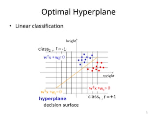
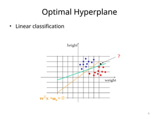
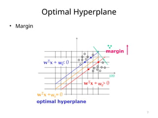
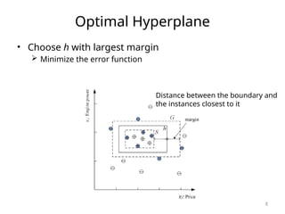
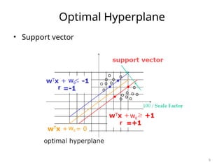
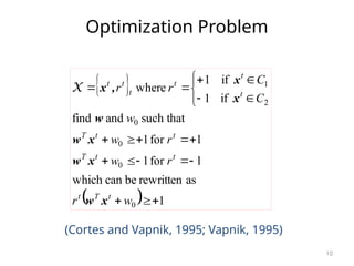
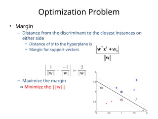
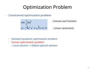
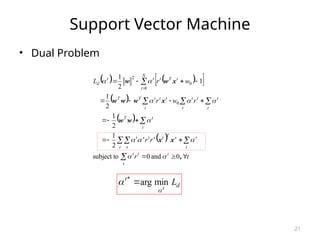
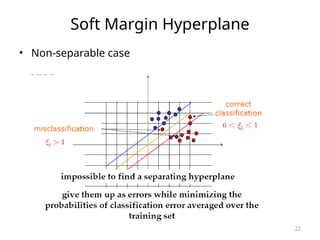
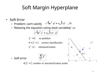
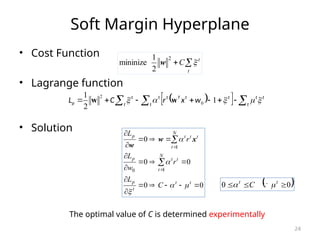
1. 1
Support Vector Machine
Part 1

2. 2
Feature Space
• Sample

3. 3
Feature Space
• Training Set
r
1
ri
r
1
r2

4. 4
Feature Space
• How to classify them using computer ?

5. 5
Optimal Hyperplane
• Linear classification
w0
w0
w0
r
r

6. 6
Optimal Hyperplane
• Linear classification
w0

7. 7
Optimal Hyperplane
• Margin
w0
w0
w0

8. 8
Optimal Hyperplane
• Choose h with largest margin
 Minimize the error function
Distance between the boundary and
the instances closest to it

9. 9
Optimal Hyperplane
• Support vector
w0
w0
w0
r
r

10. 10
Optimization Problem
(Cortes and Vapnik, 1995; Vapnik, 1995)
 
  1
as
rewritten
be
can
which
1
for
1
1
for
1
such that
and
find
if
1
if
1
where
0
0
0
0
2
1






















w
r
r
w
r
w
w
C
C
r
r
t
T
t
t
t
T
t
t
T
t
t
t
t
t
t
x
w
x
w
x
w
w
x
x
,
x
X

11. 11
Optimization Problem
• Margin
– Distance from the discriminant to the closest instances on
either side
• Distance of xt
to the hyperplane is
• Margin for support vectors
– Maximize the margin
⇒ Minimize the ||w||
w
x
w 0
w
t
T


12. 12
Optimization Problem
– Constrained optimization problem
• Standard quadratic optimization problem
• Convex optimization problem
: Local solution ⇒ Global optimal solution
  t
w
r t
T
t



 ,
x
w
w
1
s.t.
2
1
min
0
2 : Convex cost function
: Linear constraints

13. 13
Optimization Problem
• Lagrange Multipliers Method

14. 14

15. 15

16. 16

17. 17

18. 18

19. 19
Optimization Problem
• Problem
• Lagrange function (Primal)
• Solution
  t
w
r t
T
t



 ,
x
w
w
1
s.t
2
1
min
0
2
 
 
  













N
t
t
N
t
t
T
t
t
N
t
t
T
t
t
p
w
r
w
r
L
1
1
0
2
1
0
2
2
1
1
2
1



x
w
w
x
w
w
0
0
0
1
0
1














N
t
t
t
p
N
t
t
t
t
p
r
w
L
r
L

 x
w
w
 
  0
1
condition
KKT 0 


 w
x
w
r t
T
t
t


20. 20
Support Vector Machine
• Support Vector Machine (SVM) (Vapnik 1995)
 
  0
1
:
condition
KKT 0 

 w
x
w
r t
T
t
t

 
 
vector
support
not
is
0
then
1
If
vector
support
is
1
then
0
If
0
0
t
t
t
T
t
t
t
T
t
t
x
w
x
w
r
x
w
x
w
r













N
t
t
t
t
x
r
1

w : w is only related to support vectors xt
Most αt
are 0 and only a small number have αt
>0; they are the
support vectors

21. 21
Support Vector Machine
• Dual Problem
   
 
 
 
 




 




















t
0
1
0
2
0
and
0
subject to
2
1
2
1
2
1
1
2
1
t
r
r
r
r
w
r
w
r
L
t
t
t
t
t
s
T
t
s
t
t s
s
t
t
t
T
t t
t
t
t
t
t
t
t
T
T
N
t
t
T
t
t
t
d
,
x
x
w
w
x
w
w
w
x
w
w











d
t
L
t

 min
arg

*

22. 22
Soft Margin Hyperplane
• Non-separable case

23. 23
Soft Margin Hyperplane
• Soft Error
– Problem: can’t satisfy
– Relaxing the equation using slack variables
– Soft error
  t
w
r t
T
t


 ,
x
w 1
0
  t
t
T
t
w
x
r 


 1
0
w
ication
misclassif
:
1
tion
classifica
correct
:
1
0
problem
no
:
0




t
t
t



0

t


t
t

  points
ication
misclassif
of
number
:
1

t

#

24. 24
Soft Margin Hyperplane
• Cost Function
• Lagrange function
• Solution
 
  

 





 t
t
t
t
t
t
T
t
t
t
t
p w
x
r
C
L 



 1
2
1
0
2
w
w


t
t
C 
2
2
1
mininize w
0
0
0
0
0
1
0
1





















t
t
t
p
N
t
t
t
p
N
t
t
t
t
p
C
L
r
w
L
r
L




 x
w
w
 
0
0 

 t
t
C 
 
The optimal value of C is determined experimentally

25. 25
n (nu) -SVM
• Replacing C with the parameter n (Scholkopf, 2000)
– ρ : optimization variable (scales the margin),
margin size = ρ /∥w∥
– : parameter
lower bound on the fraction of support vectors
upper bound on the fraction of instances having margin errors
  0
0
subject to
1
-
2
1
min
0
2





 






,
,
x
w
w
t
t
t
T
t
t
t
w
r
N
 
1
0,












t
t
t
t
t
N
r
1
0
0
t

26. 26
Nonlinear SVM
• Nonlinear SVM
– Basis function
– Solution
   
     
x
x
φ
w
x
,
,
x
,
x
φ
z
j
k
j
j
T
j
j
w
g
k
j
z









1
1
 
       
 







t
t
t
t
t
T
t
t
t
T
t
t
t
t
K
r
r
g
r
x
,
x
x
φ
x
φ
x
φ
w
x
x
φ
w




27. 27
Nonlinear SVM

28. 28
Nonlinear SVM
 Polynomials of degree q:
   q
t
T
t
K 1

 x
x
x
x ,
   
 
   T
T
x
x
x
x
x
x
y
x
y
x
y
y
x
x
y
x
y
x
y
x
y
x
K
2
2
2
1
2
1
2
1
2
2
2
2
2
1
2
1
2
1
2
1
2
2
1
1
2
2
2
1
1
2
2
2
2
1
2
2
2
1
1
1
,
,
,
,
,
,












x
y
x
y
x

Lecture Notes for E Alpaydın 2010 Introduction to Machine Learning 2e © The MIT Press (V1.0)

29. 29
Nonlinear SVM
 Radial-basis functions:
 







 

 2
2
2s
K
t
t
x
x
x
x exp
,
Lecture Notes for E Alpaydın 2010 Introduction to Machine Learning 2e © The MIT Press (V1.0)

30. 30
Nonlinear SVM

31. 31
Nonlinear SVM

32. 32
Multiclass SVM
• Multiclass Classification
– SVM : binary classification
– Multiclass SVM: multiple binary classification
• One-to-rest vs. one-to-one
1) One-to-rest
• I 번째 class 와 I 클래스를 제외한 나머지 M-1 클래스로 이진 분류
• M 개의 이진 분류 SVM 을 학습하여 사용
2) One-to-one
• M 개의 클래스 중 2 개를 선택하여 이진 분류
• M(M-1)/2 개의 이진 분류 SVM 을 학습하여 사용

33. 33

34. 34
SVM Demo
https://jgreitemann.github.io/svm-demo

35. 35
SVM Summary
• Optimal separating hyperplane : max. margin
• Global solution (convexity)
• Analytic solution
• Model selection problem: kernel selection
• Classification & Regression 문제에 모두 적용