SlideShare a Scribd company logo
1 of 34
1
ECE, VDIT, Haliyal
Aim: To simulate a second order system and find the time domain specifications of the second order
system (subjected to unit step input), namely, a) %age peak overshoot Mp b) Peak time tp c) Rise time
tr d) Settling time ts.
Apparatus:
Equipment’s Quantity
Decade resistance box 01
Decade Capacitance box 01
Decade Inductance box 01
Signal generator 01
CRO 01
BNC 02
Patch cords 10
Theory:
In a second order system (RLC series circuit) subjected to unit step input, the output response follows
the input and attains unit value at steady state. In under damped system i.e. damping ratio (ξ< 1), the
output response C(t) exhibits oscillations exponentially decaying and settling to steady state value equal
to input as shown,





2
1
2
tan
)
sin(
1
1
)
(









 where
t
e
t
C d
t
n
Refer tr, tp, ts, Mp from the diagram. The expressions for the specifications are as follows.
2
n
d
d
r 1
where
onds
sec
.....
..........
)
t
(
time
Rise 










onds
sec
.........
..........
)
t
(
time
Peak
d
p 



%
..........
100
100
)
(
% )
(
))
(
(
1 2




 





C
C
t
C
p
p
e
M
overshoot
Peak
age 

Study and verification of step response of standard second order system (both analog and
digital system), (MATLAB), for the cases of undamped, under damped and critically, damped cases.
EXPERIMENT: 01:
2
ECE, VDIT, Haliyal
%)
2
(
onds
sec
.........
..........
4
)
t
(
time
Settling
%)
5
(
onds
sec
.........
..........
3
)
t
(
time
Settling
n
s
n
s






L
C
2
R
ξ
LC
1
ω
(2)
and
(1)
equation
Comparing
)
2
(
2
prototype
order
2
Function
Transfer
)
1
(
1
1
)
(
)
(
V
Function
Transfer
is
function
transfer
the
circuit,
series
RLC
namely
system
order
second
a
For
n
2
2
2
nd
2
o





































n
n
n
i
S
S
LC
S
L
R
S
LC
S
V
S



With increase in resistance, ξ increases where the oscillations are damped. At ξ = 1, the system is
said to be critically damped, where the oscillations are completely damped out. For ξ >1, the
system is said to be over-damped. For ξ=0, the system is said to undamped where sustained
oscillations are produced.
Procedure :-
1) Choose L=10mH, C=0.01uF arbitrarily. Calculate value of n & R for ξ=1 and ξ=1.5 respectively.
Calculate theoretical values of tp,ts,tr,Mp with each case.
2) Apply a square wave input of 1 V (p-p) .Calibrate the CRO for time scale and amplitude scale.
Adjust the resistance for ξ=0.2 i.e. under damped case. Note the corresponding response on CRO.
Measure tp, tr, ts, Mp. Compare the measured quantities with the theoretical values, for verification.
3) Similarly adjust R for ξ=1, critically damped case. Note the corresponding response on CRO.
Measure ts.
4) Also for ξ=0.5, adjust R correspondingly for Over damped case . Note the corresponding response
on CRO. Measure only ts.
5) On graph sheet plot the response showing the quantities measured. Practically ξ=0, undamped
case cannot be simulated as L & C elements have certain finite resistance.
3
ECE, VDIT, Haliyal
Observations: -
Sl.
No
R in
Ω s
Ξ
tp in
sec
Tp
sec
Tr
Sec
Tr
sec
Ts
sec
Ts
sec
Mp in
%
age
Mp in
%
age
Actual Cal Actual Cal Actual Cal Actual Cal
01 200 0.1
02 2000 1.0
03 3000 1.5
Conclusion:-
Write briefly about system response in each case of damping. Compare the settling times in each case.
Calculations:
The second order standard transfer function is given by.
T. F =
CIRCUIT DIAGRAM
4
ECE, VDIT, Haliyal
MATLAB PROGRAM
wn= input('frequency')
zeta= input('damping factor')
k= input('constant')
num= [k*wn^2]
deno= [1 2*zeta*wn wn^2]
g= tf(num, deno)
t= feedback(g,1)
step(t, 'r')
Example :
5
ECE, VDIT, Haliyal
Aim:- To design a passive RC lead-lag compensating network for the specified maximum
phase lead angle Фm and ωm, the frequency at which it occurs i.e. ωm and then determine it’s
frequency Bode diagrams. Using the Bode diagrams, determine the transfer function of the lead
compensating network
Apparatus:-
Equipments
Quantity
Decade resistance
box
02
Decade Capacitance
box
01
Signal generator 01
CRO 01
BNC 02
Patch cords 10
Theory:-
Lead compensating network is used in control systems to stabilize unstable systems or to
improve relative stability by improving gain margin and phase margin. Lead compensator used as
series compensator has the following effects on the system performance. (Refer figure 1).
a) Increase in bandwidth and speed of response.
b) Decrease in maximum overshoot in response
c) Improvement in relative stability with increase in PM.
d) Acts as high pass filter attenuating low frequency signals and hence useful in low damped systems.
To design a Lag-Lead compensator and to obtain the characteristics by simulation using MATLAB.
Verify the performance using experiments with the compensator circuit made of passive elements
EXPERIMENT: 02
6
ECE, VDIT, Haliyal
Circuit Diagram :
Characteristics:
Design of passive RC lead compensating network
From the specifications, it is desired to obtain maximum phase lead Фm =____________ at
a frequency F=__________Hz ωm= 2ΠF=_________ rad/sec.
1. From
1
a
1
a
sin m



 , find ‘a’ substituting Фm.
2. From
d
m
a
1


 ,find Td substituting ωm and a.
7
ECE, VDIT, Haliyal
3. Assume C = 0.1μF
4. Determine R1 and R2.
But,
2
2
1
d
n
n
2
1
2
2
1
2
1
d
1
n
R
R
R
a
R
R
R
)
R
R
/(
C
R
R
and
C
R













Design Calculations: for Φm=……….. degrees ωm=………..rad/sec.
Procedure:
1. Rig up the designed lead compensating network as shown.
2. Using signal generator, apply sinusoidal input signal (about 2V p-p ) with the frequency varying
over a wide range from 20 Hz to 300 kHz.
3. Increase the frequency of the input signal gradually and at each frequency note down peak to peak
amplitude of input and output signals. Also note down the phase difference between the i/p and
o/p signals using Lissageous pattern on CRO.
4. Maintain the amplitude of i/p signal constant at all frequencies.
5. Plot Bode’s magnitude and phase plots on semi log sheet.
Observations:
I/P signal (p-p) = 2V
Frequency
in Hz
Input
Voltage Vi
Output
Voltage Vo
AB XY Gain in db =
20 log(Vo/Vi)
Ф = sin (AB/XY)
8
ECE, VDIT, Haliyal
Lissageous pattern
MATLAB PROGRAM
clc;close all;clear;
%transfer function
s=tf('s');
G=0.2/(s*(s+1));
%Root locus
rlocus(G);
%calculate the Shortage Phase
syms s1
G1=0.2/(s1*(s1+1));
phi=double(angle(subs(G1,s1,-4+6.93i)))*180/pi;
sphi=180-phi;
%T , a
z=-4;
p=-4-6.93/tand(90-sphi);
%shart andazeh
Gc1=(s1-z)/(s1-p);
kc=1/(double(abs(subs(Gc1*G1,-4+6.93i))));
%simulation
Gc=(s-z)/(s-p);
Gcloseloop=kc*Gc*G/(1+kc*Gc*G);
figure;
rlocus(Gc*G);
Attach Printout of Program
9
ECE, VDIT, Haliyal
EXPERIMENT: 03:
Steady state error analysis for Type-0, Type-1, Type-2 digital control system using MATLAB by
applying standard reference inputs of step , ramp and parabola.
.
A MATLAB program which will get the transfer function of the system and returns the following.
a. System type as a string (Type 0 or Type 1 or Type 2)
b. Steady state error for
i. Step input
ii. Ramp input
iii. Parabolic input
A system is called type 0, type 1, type 2,p , if N=0, N=1, N=2, p , respectively. Note that this classification is
different from that of the order of a system. As the type number is increased, accuracy is improved; however,
increasing the type number aggravates the stability problem. A compromise between steady-state accuracy
and relative stability is always necessary.
MATLAB PROGRAM
clc;
close all;
clear all;
h1=h2=h3=1;
g1=zpk([-3 -5],[-7 -8],[1]);
g2=zpk([-3 -5],[0 -7 -8],[1]);
g3=zpk([-3 -5],[0 0 -7 -8],[1]);
chk1=find(pole1==0);
chk2=find(pole2==0);
chk3=find(pole3==0);
x1=length(chk1);
x2=length(chk2);
x3=length(chk3);
fprintf('System 1 if of type %dn',x1);
fprintf('System 2 if of type %dn',x2);
fprintf('System 3 if of type %dn',x3);
s=tf('s');
kp1=dcgain(g1*h1);
kv1=dcgain(s*g1*h1);
ka1=dcgain((s^2)*g1*h1);
kp2=dcgain(g2*h2);
kv2=dcgain(s*g2*h2);
ka2=dcgain((s^2)*g2*h2);
kp3=dcgain(g3*h3);
10
ECE, VDIT, Haliyal
kv3=dcgain(s*g3*h3);
ka3=dcgain((s^2)*g3*h3);
e1_step=1/(1+kp1);
e1_ramp=1/kv1;
e1_para=1/ka1;
e2_step=1/(1+kp2);
e2_ramp=1/kv2;
e2_para=1/ka2;
e3_step=1/(1+kp3);
e3_ramp=1/kv3;
e3_para=1/ka3;
ATTACH THE OUTPUT PRINTOUT
11
ECE, VDIT, Haliyal
Design a digital controller with output feedback to control the speed of a DC motor; simulate the
design using Simulink.
EXPERIMENT: 04
AIM: To simulate a DC position control system using armature controlled DC motor in MATLAB and
obtain its step response through state space approach for i) open loop ii) closed loop operations
THEORY:
a) Consider an armature controlled DC motor open loop position control system.
From the state equations the state model is
12
ECE, VDIT, Haliyal
From the state model
Take KT = 1 Nm/Amp, Kb = 1 Volts/radians/sec, J = 4×10⁻³ Nm/radians/sec,
Ra = 5Ώ, La = 1mH and f=2x10⁻³. Simulate the state space model in MATLAB to obtain its step
response.
% step response of open loop DC position control system
f = 0.002; Kb = 1; La = 0.001; Ra = 5; KT = 1;
Kb=1; J=4e-3;
title (‘Step Response of open Loop DC position Control System’);
13
ECE, VDIT, Haliyal
MATLAB PROGRAM
t = 0:0.1:15;
Td = -0.1 * (t>5 & t<10); % load disturbance
u = [ones(size(t)) ; Td]; % w_ref=1 and Td
cl_ff = dcm * diag([Kff,1]); % add feedforward gain
cl_ff.InputName = {'w_ref','Td'};
cl_ff.OutputName = 'w';
h = lsimplot(cl_ff,u,t);
title('Setpoint tracking and disturbance rejection')
legend('cl_ff')
% Annotate plot
line([5,5],[.2,.3]);
line([10,10],[.2,.3]);
text(7.5,.25,{'disturbance','T_d = -0.1Nm'},...
'vertic','middle','horiz','center','color','r');
Expected Output
14
ECE, VDIT, Haliyal
A linear model of the system can be extracted from the Simulink model into the MATLAB workspace. This can be
accomplished employing the MATLAB command linmod or from directly within Simulink as we will do here. We
will specifically use the base Simulink model developed from first principles shown below. You can download this
model by right-clicking here and then selecting Save link as ..., or you can refer to the DC Motor Speed: Simulink
Modeling page to recreate the model yourself.
Recall that the physical parameters have to be set if they have not previously been defined in the workspace.
J = 0.01;
b = 0.1;
K = 0.01;
R = 1;
L = 0.5;
Design a digital controller with state variable feedback to control the speed of a DC motor;
simulate the design using Simulink
EXPERIMENT: 05
15
ECE, VDIT, Haliyal
We then need to identify the inputs and outputs of the model we wish to extract. First right-click on the signal
representing the Voltage input in the Simulink model. Then choose Linear Analysis Points > Open-loop
Input from the resulting menu. Similarly, right-click on the signal representing the Speed output and select Linear
Analysis Points > Open-loop Output from the resulting menu. The input and output signals should now be
identified on your model by arrow symbols as shown in the figure below.
In order to perform the extraction, select from the menus at the top of the model window Analysis > Control
Design > Linear Analysis. This will cause the Linear Analysis Tool to open. Within the Linear Analysis
Tool window, the Operating Point to be linearized about can remain the default, Model Initial Condition. In order
to perform the linearization, next click the Step button identified by a step response with a small green triangle. The
result of this linearization is the linsys1 object which will appear in the Linear Analysis Workspace as shown
below. Furthermore, the open-loop step response of the linearized system also will be generated automatically.
The open-loop step response above is consistent with the response generated in the DC Motor Speed: System
Analysis page The reason the responses match so closely is because this Simulink model uses only linear
components. Note that this process can be used to extract linear approximations of models with nonlinear elements
too.
We will further verify the model extraction by looking at the model itself. The linearized model can be exported by
simply dragging the object into the MATLAB Workspace. This object can then be used within MATLAB in the
same manner as an object created directly from the MATLAB command line. Specifically, entering the
command zpk(linsys1) in the MATLAB command window demonstrates that the resulting model has the following
form.(1)
16
ECE, VDIT, Haliyal
This model matches the one generated in the DC Motor Speed: System Modeling page. This can be seen by
repeating the MATLAB commands given below.
s = tf('s');
P_motor = K/((J*s+b)*(L*s+R)+K^2);
zpk(P_motor)
ans = 2
-------------------
(s+9.997) (s+2.003)
Open-loop response
The open-loop step response can also be generated directly within Simulink, without extracting any models to the
MATLAB workspace. In order to simulate the step response, the details of the simulation must first be set. This can
be accomplished by selecting Model Configuration Parameters from the Simulation menu. Within the resulting
menu, define the length for which the simulation is to run in the Stop time field. We will enter "3" since 3 seconds
will be long enough for the step response to reach steady state. Within this window you can also specify various
aspects of the numerical solver, but we will just use the default values for this example.
Next we need to add an input signal and a means for displaying the output of our simulation. This is done by doing
the following:
 Remove the In1 and Out1 blocks.
 Insert a Step block from the Simulink/Sources library and connect it with a line to the Voltage input of the motor
subsystem.
 To view the Speed output, insert a Scope from the Simulink/Sinks library and connect it to the Speed output of
the motor subsystem.
 To provide an appropriate unit step input at t=0, double-click the Step block and set the Step time to "0".
The final model should appear as shown in the following figure.
Then run the simulation (press Ctrl-T or select Run from the Simulation menu). When the simulation is finished,
double-click on the scope and you should see the following output.
17
ECE, VDIT, Haliyal
This response is identical to that obtained by MATLAB above using the extracted model. This is again to be
expected because this Simulink model includes only linear blocks.
Closed-loop response with lag compensator
In the DC Motor Speed: Root Locus Controller Design page a lag compensator was designed with the following
transfer function. (2)
To generate the closed-loop step response with this compensator in Simulink, we will begin with the
"Motor_Model.slx" file described above. We will then put the lag compensator in series with the motor subsystem
and will feed back the motor's speed for comparison to a desired reference.
More specifically, follow the steps given below:
 Remove the Input and Output ports of the model.
 Insert a Sum block from the Simulink/Math Operations library. Then double-click on the block and enter "|+-"
for its List of signs where the symbol "|" serves as a spacer between ports of the block.
 Insert a Transfer Function block from the Simulink/Continuous library. Then double-click on the block and edit
the Numerator coefficients field to "[44 44]" and the Denominator coefficients field to "[1 0.01]".
 Insert a Step block from the Simulink/Sources library. Then double-click on the block and set the Step time to
"0".
 Insert a Scope block from the Simulink/Sinks library.
Then connect and label the components as shown in the following figure
18
ECE, VDIT, Haliyal
You can download our version of the closed-loop system model by right-clicking here and then selecting Save link
as ....
Then run the simulation (press Ctrl-T or select Run from the Simulation menu). When the simulation is finished,
double-click on the scope and you should see the following output.
This step response matches exactly the closed-loop performance observed in the DC Motor Speed: Root Locus
Controller Design page where the lag compensator was originally designed. Note that while we used the physics-
based Simulink model developed in the DC Motor Speed: Simulink Modeling page for simulating the closed-loop
system, we could have equivalently used the Simscape version of the DC motor model.
Closed-loop response with lead compensator
We have shown in the above and in other pages of this example that the lag compensator we have designed meets
all of the given design requirements. Instead of a lag compensator, we could have also designed a lead compensator
to meet the given requirements. More specifically, we could have designed a lead compensator to achieve a similar
DC gain and phase margin to that achieved by the lag compensator, but with a larger gain crossover frequency. You
can refer back to the DC Motor Speed: Frequency Domain Methods for Controller Design page for more details on
19
ECE, VDIT, Haliyal
the design of the lag compensator, but the fact that the DC gains and phase margins are similar indicate that the
responses under lag and lead control would have similar amounts of error in steady state and similar amounts of
overshoot. The difference in response would come in that the larger gain crossover frequency provided by the lead
compensator would make the system response faster than with the lag compensator. We will specifically use the
following lead compensator.(3)
To see the precise effect of the lead compensator as compared to our lag compensator, let's modify our Simulink
model from above as follows:
 Disconnect the Step block and Scope block from the rest of the model.
 Copy the blocks forming the closed-loop of the model: the Sum block, the Transfer Function block, and the DC
Motor subsystem. Then paste a copy of this loop below the original blocks.
 Double-click on the Transfer Function block and edit the Numerator coefficients field to "[160000 5.6e6]" and
the Denominator coefficients field to "[1 1035]".
 Insert a Mux block from the SimulinkSignal Routing library and connect the outputs of the two Motor
subsystem blocks to the inputs of the Mux and connect the output of the Mux to the Scope.
 Connect the Step block to the Sum block of the original feedback system. Then branch off from this line and
connect it to the Sum block of the lead compensated system as well.
The Mux block serves to bundle the two signals into a single line, this way the Scope will plot both speed signals on
the same set of axes. When you are done, your model should appear as follows.
Running the simulation and observing the output produced by the scope, you will see that both responses have a
steady-state error that approaches zero. Zooming in on the graphs you can generate a figure like the one shown
below. Comparing the two graphs, the blue response belonging to the lead compensated system has a much smaller
settle time and slightly larger, but similar, overshoot as compared to the yellow response produced by the lag
compensated system.
20
ECE, VDIT, Haliyal
It is generally preferred that a system respond to a command quickly. Why then might we prefer to use the lag
compensator even though it is slower than the lead compensator? The advantage of the lag compensator in this case
is that by responding more slowly it requires less control effort than the lead compensator. Less control effort means
that less power is consumed and that the various components can be sized smaller since they do not have to supply
as much energy or withstand the higher voltages and current required of the lead compensator.
We will now modify our simulation to explicitly observe the control effort requirements of our two feedback
systems. We will do this by sending our various signals to the workspace for plotting and further manipulation if
desired. Specifically, delete the Scope and Mux blocks from your Simulink model. Then insert four To Workspace
blocks from the SimulinkSinks library. Double-click on each of the blocks and change their Save
format from Structure to Array. Also provide a Variable name within each block that will make sense to you. You
can then connect the blocks to the existing model and label them as shown below. You can download our version of
this Simulink model by right-clicking here and then selecting Save link as ....
21
ECE, VDIT, Haliyal
Then change the simulation stop time to 1 second and run the model. The act of running the simulation will send to
the MATLAB workspace a series of arrays corresponding to the variables set-up in your model with the To
Workspace blocks. Furthermore, the time vector used by that run of the simulation is stored in the default
variable tout. You can now plot the results of your simulation from the workspace. Enter the following code to see
how to specifically plot the control effort variables.
subplot(2,1,1)
plot(tout,ulag);
xlabel('time (seconds)')
ylabel('control effort (volts)')
title('Control Effort Under Lag Compensation')
subplot(2,1,2)
plot(tout,ulead);
xlabel('time (seconds)')
ylabel('control effort (volts)')
title('Control Effort Under Lead Compensation')
22
ECE, VDIT, Haliyal
This example shows how to use numerical optimization to tuning the controller parameters of a nonlinear system. In
this example, we model a CE 152 Magnetic Levitation system where the controller is used to position a freely
levitating ball in a magnetic field. The control structure for this model is fixed and the required controller
performance can be specified in terms of an idealized time response.
Earnshaw's Theorem
Earnshaw's theorem proved that it is not possible to achieve stable levitation using static, macroscopic, classical
electromagnetic fields. However the CE 152 system works around this by creating a potential well around the point
at which the ball is to be suspended, thereby creating a non-inverse square law force. This is achieved by an
inductive coil that generates a time varying electromagnetic field. The electromagnetic field is controlled through
the use of feedback to keep the ball at the required location.
open_system('maglev_demo')
Design a digital controller with output feedback to control the position of the metallic ball in
Magnetic levitation experiment and simulate the design using Simulink
EXPERIMENT: 06
23
ECE, VDIT, Haliyal
Model Description
The magnetic levitation system is a nonlinear dynamic system with one input and one output. Double-click
the Magnetic Levitation Plant Model to open this subsystem. The input voltage is applied to a coil that creates the
electromagnetic field. The output voltage is measured by an IR receiver and represents the position of the ball in the
magnetic field. The diagram below outlines this system.
The physical system consists of a ball (with mass 0.00837 kg) which is under the influence of three forces:
 The magnetic field produced by an inductive coil. This is modeled by the Power amplifier and coil block in the
Simulink® model. The input to the inductor is a voltage signal and the output a current. The force from the coil
depends on the square of the current, the air-gap between the coil and the ball, and the physical properties of the
ball. This produces an upward acting force on the ball.
 The gravitational force acting downwards
 A damping force which acts in a direction opposite to the velocity at any instant of time
These three forces cause the resulting motion of the ball and are modeled in Simulink as shown.
open_system('maglev_demo/Magnetic Levitation Plant Model')
24
ECE, VDIT, Haliyal
Non-linearities arising from saturation of the coil and changes in dynamics outside the limits of the magnetic field
are also modeled in the Simulink Model. As the force from the coil decays according to an inverse square law larger
voltages are required the further the ball is from the coil. The control signal is scaled to account for this and the
scaling is included in the Control signal scaling blocks.
Control Problem Description
The requirement for the controller is that it be able to position the ball at any arbitrary location in the magnetic field
and that it move the ball from one position to another. These requirements are captured by placing step response
bounds on the position measurement. Specifically we require the following constraints on the ball:
 Position constraint: within 20% of the desired position in less than 0.5 second
 Settling Time Constraint: within 2% of the desired position within 1.5 second
To meet the control requirements we implement a Proportional-Integral-Derivative (PID) controller. For
convenience the controller uses a normalized position measurement with a range from 0 to 1, representing the
bottom-most and top-most positions of the ball respectively.
Simulink® Design Optimization™ and numerical optimization is ideally suited to tune the PID coefficients
because:
 The system dynamics are complex enough to require effort and time for analysis if we approach the problem
using conventional control design techniques.
 The controller structure is fixed.
 We have knowledge of the step response we require from the system.
Setting Constraint Values
Given the step response characteristic we desire, it is simple to specify the upper and lower bounds of the response.
Double-click the Position Constraint block in the Magnetic Levitation Plant Model subsystem to view constraints
on the position of the ball. The constraint lines may be moved using the mouse.
25
ECE, VDIT, Haliyal
You can launch the Response Optimizer using the Apps menu in the Simulink toolstrip, or the sdotool command
in MATLAB®. You can launch a pre-configured optimization task in the Response Optimizer by first opening the
model and by double-clicking on the orange block at the bottom of the model. From the Response Optimizer, press
the Plot Model Response button to simulate the model and show how well the initial design satisfies the design
requirements.
Defining Tuned Parameters
26
ECE, VDIT, Haliyal
We select the PID controller parameters to tune by opening the Design Variables editor, as shown below.
Running the Optimization
After specifying the optimization parameters and the required step response bounds we start the optimization by
pressing the Optimize button from the Response Optimizer. During optimization, the plots are updated with the
position of the ball for each iteration and the dark curve shows the final optimized trajectory of the ball (as shown
below).
27
ECE, VDIT, Haliyal
Verifying the Results
Once we complete the optimization, it is important to validate the results against other step sizes. A successful
parameter optimization should be able to provide good control for all steps sizes close to the tuned step size of 1.
Step sizes from .7 to 1 should be tested to confirm the controller's performance. The following plot shows the
response to a step input from 0 to 0.85 at 0.1 seconds.
Conclusion
The verification step shows that controller's performance satisfies the requirements specified and the tuned
parameter values are suitable for control. The tuned parameters could be used to provide baseline performance
against which other control schemes can be compared, or a baseline for controllers for different operating regions.
% Close the model.
bdclose('maglev_demo')
28
ECE, VDIT, Haliyal
Equipment needed
 Arduino board (e.g. Uno, Mega 2560, etc.)
 lightbulb (incandescent, LED, CFL, etc.)
 AC solid-state relay (hockey-puck type, etc.)
 temperature sensor (TMP36, etc.)
The temperature of the lightbulb is measured in this example with a TMP36 sensor (cheap, relatively accurate,
sufficient range). The Arduino board provides power to the sensor and reads the sensor output via an Analog Input.
The Arduino board is also used for generating the Digital Output that switches the solid-state relay on and off. That
is, the digital output alternately connects and disconnects the light bulb from the AC power source (from the wall)
via the relay in order to turn the light bulb on and off. The control logic employed for determining when to switch
the relay on and off is implemented within Simulink, which is also employed for visualizing the light bulb's
temperature and the control signal.
System identification experiment
In order to implement our temperature control system, we technically don't need a model of our plant (the light
bulb). We can simply employ logic that turns the light bulb on when the measured temperature is lower than desired
and turns the light bulb off when the temperature is higher than desired. We, however, would like to be able to
explain the resulting behavior of our control system (and perhaps even attempt to design the control algorithm in a
more intelligent manner). Therefore, we will generate a model for the thermal behavior of the light bulb based on its
observed response. This is sometimes referred to as a blackbox model or a data-driven model. After we have
generated such a model, we will attempt to explain what we have observed based on our understanding of the
underlying physics.
Hardware setup
In this experiment our plant is a standard incandescent light bulb where we will (ultimately) attempt to control the
light bulb's temperature. We have chosen a 25 W bulb in order to keep the maximum temperature within the limits
of the temperature sensor we have chosen. You can also employ other types of bulbs (LED, CFL, etc.).
For our temperature sensor, we will employ the TMP36 (though many others can be employed). This sensor
measures temperature in Celsius, is quite inexpensive (a couple of dollars), has adequate range, reasonable
accuracy, and doesn't need to be calibrated. This sensor is also commonly included in many Arduino starter kits that
are in the market place. The datasheet for this sensor can be found here. The temperature sensor can be attached to
the surface of the lightbulb employing thermally conductive epoxy, or with adhesive metal tape. The TMP36 is
connected to the Arduino Board as shown below. Specifically, if the sensor is oriented such that the pins are pointed
downward and the flat side of the sensor is facing you, then the leftmost pin is the power (must be between 2.7 V
and 5.5 V), the middle pin is the signal, and the rightmost pin is ground. Power and ground for the TMP36 are
supplied from the Arduino board and the signal, which is a voltage that is linearly proportional to temperature, is
read on one of the board's Analog Inputs.
Implement an on-off temperature controller to control lamp using a temperature sensor and
dspace DS1104 hardware interface
EXPERIMENT: 07
29
ECE, VDIT, Haliyal
The lightbulb is turned on and off employing a digital output from the Arduino board via a solid-state relay. The
solid-state relay is basically an electrical switch that can connect/disconnect a (possibly high-power) device to an
AC source with a low-power DC signal. In our case, the AC source comes from a standard wall outlet and the DC
signal is supplied by a Digital Output from our Arduino board. Therefore, our solid-state relay needs to be able to
handle 120-240 V on the AC side (in North America need 120 V) and the DC side must be able to be controlled
with a 5 V signal. Since our load (the lightbulb) is resistive (not inductive) and doesn't require much current, we
don't have to be very particular about the solid-state relay we employ. We are in particular employing a simple
"hockey-puck" style relay. In order to control the lightbulb, we need to insert the relay into the circuit (the loop) that
connects the lightbulb to the wall. Therefore, we must cut into the cord for the lightbulb and wire the relay into the
circuit. In doing this, make sure that the bulb is not plugged in. You should insert the relay on the neutral wire of the
bulb's plug. The neutral wire is indicated by a white stripe or ribbing. If you insert the relay on the live wire, then
the terminals of the relay are connected to the power supply even when the relay is off. You should also cover the
exposed terminals of the relay and never touch the terminals when the bulb is plugged in.
30
ECE, VDIT, Haliyal
MAT LAB PROGRAM
s = tf('s');
To = 18.5; % ambient/initial temperature
K = 83.5; % DC gain
tau = 66; % time constant
P = K/(tau*s+1); % model transfer function
[y,t] = step(P,350); % model step response
plot(t+50,y+To);
hold
plot(temp,'r:')
xlabel('time (sec)')
ylabel('temperature (degrees C)')
title('Lightbulb Temperature Step Response')
legend('model','experiment','Location','SouthEast')
EXPECTED OUTPUT
31
ECE, VDIT, Haliyal
Equipment needed
 Arduino board (e.g. Uno, Mega 2560, etc.)
 lightbulb (incandescent, LED, CFL, etc.)
 AC solid-state relay (hockey-puck type, etc.)
 temperature sensor (TMP36, etc.)
The temperature of the lightbulb is measured in this example with a TMP36 sensor (cheap, relatively accurate,
sufficient range). The Arduino board provides power to the sensor and reads the sensor output via an Analog Input.
The Arduino board is also used for generating the Digital Output that switches the solid-state relay on and off. That
is, the digital output alternately connects and disconnects the light bulb from the AC power source (from the wall)
via the relay in order to turn the light bulb on and off. The control logic employed for determining when to switch
the relay on and off is implemented within Simulink, which is also employed for visualizing the light bulb's
temperature and the control signal.
System identification experiment
In order to implement our temperature control system, we technically don't need a model of our plant (the light
bulb). We can simply employ logic that turns the light bulb on when the measured temperature is lower than desired
and turns the light bulb off when the temperature is higher than desired. We, however, would like to be able to
explain the resulting behavior of our control system (and perhaps even attempt to design the control algorithm in a
more intelligent manner). Therefore, we will generate a model for the thermal behavior of the light bulb based on its
observed response. This is sometimes referred to as a blackbox model or a data-driven model. After we have
generated such a model, we will attempt to explain what we have observed based on our understanding of the
underlying physics.
Hardware setup
In this experiment our plant is a standard incandescent light bulb where we will (ultimately) attempt to control the
light bulb's temperature. We have chosen a 25 W bulb in order to keep the maximum temperature within the limits
of the temperature sensor we have chosen. You can also employ other types of bulbs (LED, CFL, etc.).
For our temperature sensor, we will employ the TMP36 (though many others can be employed). This sensor
measures temperature in Celsius, is quite inexpensive (a couple of dollars), has adequate range, reasonable
accuracy, and doesn't need to be calibrated. This sensor is also commonly included in many Arduino starter kits that
are in the market place. The datasheet for this sensor can be found here. The temperature sensor can be attached to
the surface of the lightbulb employing thermally conductive epoxy, or with adhesive metal tape. The TMP36 is
connected to the Arduino Board as shown below. Specifically, if the sensor is oriented such that the pins are pointed
downward and the flat side of the sensor is facing you, then the leftmost pin is the power (must be between 2.7 V
and 5.5 V), the middle pin is the signal, and the rightmost pin is ground. Power and ground for the TMP36 are
supplied from the Arduino board and the signal, which is a voltage that is linearly proportional to temperature, is
read on one of the board's Analog Inputs.
The lightbulb is turned on and off employing a digital output from the Arduino board via a solid-state relay. The
solid-state relay is basically an electrical switch that can connect/disconnect a (possibly high-power) device to an
Design a digital controller with output feedback to control the speed of a DC motor; Control the
DC motor using dspace DS1104 hardware interface
EXPERIMENT: 08
32
ECE, VDIT, Haliyal
AC source with a low-power DC signal. In our case, the AC source comes from a standard wall outlet and the DC
signal is supplied by a Digital Output from our Arduino board. Therefore, our solid-state relay needs to be able to
handle 120-240 V on the AC side (in North America need 120 V) and the DC side must be able to be controlled
with a 5 V signal. Since our load (the lightbulb) is resistive (not inductive) and doesn't require much current, we
don't have to be very particular about the solid-state relay we employ. We are in particular employing a simple
"hockey-puck" style relay. In order to control the lightbulb, we need to insert the relay into the circuit (the loop) that
connects the lightbulb to the wall. Therefore, we must cut into the cord for the lightbulb and wire the relay into the
circuit. In doing this, make sure that the bulb is not plugged in. You should insert the relay on the neutral wire of the
bulb's plug. The neutral wire is indicated by a white stripe or ribbing. If you insert the relay on the live wire, then
the terminals of the relay are connected to the power supply even when the relay is off. You should also cover the
exposed terminals of the relay and never touch the terminals when the bulb is plugged in.
33
ECE, VDIT, Haliyal
MAT LAB PROGRAM
s = tf('s');
To = 18.5; % ambient/initial temperature
K = 83.5; % DC gain
tau = 66; % time constant
P = K/(tau*s+1); % model transfer function
[y,t] = step(P,350); % model step response
plot(t+50,y+To);
hold
plot(temp,'r:')
xlabel('time (sec)')
ylabel('temperature (degrees C)')
title('Lightbulb Temperature Step Response')
legend('model','experiment','Location','SouthEast')
EXPECTED OUTPUT
34
ECE, VDIT, Haliyal

More Related Content

Similar to Digital Controller Design for DC Motor Speed Control

EE411 lecture 13- Design of Compensators in Frequency Domain.pptx
EE411  lecture 13- Design of Compensators in Frequency Domain.pptxEE411  lecture 13- Design of Compensators in Frequency Domain.pptx
EE411 lecture 13- Design of Compensators in Frequency Domain.pptxmonaibrahim598401
 
STEP RESPONSE OF FIRST ORDER SYSTEM PART 1.pptx
STEP RESPONSE OF FIRST ORDER SYSTEM PART 1.pptxSTEP RESPONSE OF FIRST ORDER SYSTEM PART 1.pptx
STEP RESPONSE OF FIRST ORDER SYSTEM PART 1.pptxAnikendu Maitra
 
CAPACITIVE SENSORS ELECTRICAL WAFER SORT
CAPACITIVE SENSORS ELECTRICAL WAFER SORTCAPACITIVE SENSORS ELECTRICAL WAFER SORT
CAPACITIVE SENSORS ELECTRICAL WAFER SORTMassimo Garavaglia
 
IC Design of Power Management Circuits (III)
IC Design of Power Management Circuits (III)IC Design of Power Management Circuits (III)
IC Design of Power Management Circuits (III)Claudia Sin
 
PSpiceで位相余裕度シミュレーション
PSpiceで位相余裕度シミュレーション PSpiceで位相余裕度シミュレーション
PSpiceで位相余裕度シミュレーション Tsuyoshi Horigome
 
HW3 – Nichols plots and frequency domain specifications FORM.docx
HW3 – Nichols plots and frequency domain specifications FORM.docxHW3 – Nichols plots and frequency domain specifications FORM.docx
HW3 – Nichols plots and frequency domain specifications FORM.docxsheronlewthwaite
 
Feedback control of_dynamic_systems
Feedback control of_dynamic_systemsFeedback control of_dynamic_systems
Feedback control of_dynamic_systemskarina G
 
Design and implementation of cyclo converter for high frequency applications
Design and implementation of cyclo converter for high frequency applicationsDesign and implementation of cyclo converter for high frequency applications
Design and implementation of cyclo converter for high frequency applicationscuashok07
 
Lab 9 Frequency response lecture file.pdf
Lab 9 Frequency response lecture file.pdfLab 9 Frequency response lecture file.pdf
Lab 9 Frequency response lecture file.pdfalfqythythm296
 
BALLANDBEAM_GROUP7.pptx
BALLANDBEAM_GROUP7.pptxBALLANDBEAM_GROUP7.pptx
BALLANDBEAM_GROUP7.pptxOthmanBensaoud
 
Lag lead compensator design in frequency domain 7th lecture
Lag lead compensator design in frequency domain  7th lectureLag lead compensator design in frequency domain  7th lecture
Lag lead compensator design in frequency domain 7th lectureKhalaf Gaeid Alshammery
 
[D08.00015] ROBUST AND OPTIMAL CONTROL FOR SUPERCONDUCTING QUBITS, 2-QUBIT G...
[D08.00015] ROBUST AND OPTIMAL CONTROL FOR  SUPERCONDUCTING QUBITS, 2-QUBIT G...[D08.00015] ROBUST AND OPTIMAL CONTROL FOR  SUPERCONDUCTING QUBITS, 2-QUBIT G...
[D08.00015] ROBUST AND OPTIMAL CONTROL FOR SUPERCONDUCTING QUBITS, 2-QUBIT G...HarrisonBall1
 
Chapter 18
Chapter 18Chapter 18
Chapter 18Tha Mike
 
Development of Digital Controller for DC-DC Buck Converter
Development of Digital Controller for DC-DC Buck ConverterDevelopment of Digital Controller for DC-DC Buck Converter
Development of Digital Controller for DC-DC Buck ConverterIJPEDS-IAES
 
PWM Buck Converter using Average Model
PWM Buck Converter using Average ModelPWM Buck Converter using Average Model
PWM Buck Converter using Average ModelTsuyoshi Horigome
 
RF Module Design - [Chapter 7] Voltage-Controlled Oscillator
RF Module Design - [Chapter 7] Voltage-Controlled OscillatorRF Module Design - [Chapter 7] Voltage-Controlled Oscillator
RF Module Design - [Chapter 7] Voltage-Controlled OscillatorSimen Li
 

Similar to Digital Controller Design for DC Motor Speed Control (20)

EE411 lecture 13- Design of Compensators in Frequency Domain.pptx
EE411  lecture 13- Design of Compensators in Frequency Domain.pptxEE411  lecture 13- Design of Compensators in Frequency Domain.pptx
EE411 lecture 13- Design of Compensators in Frequency Domain.pptx
 
STEP RESPONSE OF FIRST ORDER SYSTEM PART 1.pptx
STEP RESPONSE OF FIRST ORDER SYSTEM PART 1.pptxSTEP RESPONSE OF FIRST ORDER SYSTEM PART 1.pptx
STEP RESPONSE OF FIRST ORDER SYSTEM PART 1.pptx
 
CAPACITIVE SENSORS ELECTRICAL WAFER SORT
CAPACITIVE SENSORS ELECTRICAL WAFER SORTCAPACITIVE SENSORS ELECTRICAL WAFER SORT
CAPACITIVE SENSORS ELECTRICAL WAFER SORT
 
IC Design of Power Management Circuits (III)
IC Design of Power Management Circuits (III)IC Design of Power Management Circuits (III)
IC Design of Power Management Circuits (III)
 
Final Project
Final ProjectFinal Project
Final Project
 
PSpiceで位相余裕度シミュレーション
PSpiceで位相余裕度シミュレーション PSpiceで位相余裕度シミュレーション
PSpiceで位相余裕度シミュレーション
 
NASA 2004 PP
NASA 2004 PPNASA 2004 PP
NASA 2004 PP
 
HW3 – Nichols plots and frequency domain specifications FORM.docx
HW3 – Nichols plots and frequency domain specifications FORM.docxHW3 – Nichols plots and frequency domain specifications FORM.docx
HW3 – Nichols plots and frequency domain specifications FORM.docx
 
Feedback control of_dynamic_systems
Feedback control of_dynamic_systemsFeedback control of_dynamic_systems
Feedback control of_dynamic_systems
 
Design and implementation of cyclo converter for high frequency applications
Design and implementation of cyclo converter for high frequency applicationsDesign and implementation of cyclo converter for high frequency applications
Design and implementation of cyclo converter for high frequency applications
 
Lab 9 Frequency response lecture file.pdf
Lab 9 Frequency response lecture file.pdfLab 9 Frequency response lecture file.pdf
Lab 9 Frequency response lecture file.pdf
 
BALLANDBEAM_GROUP7.pptx
BALLANDBEAM_GROUP7.pptxBALLANDBEAM_GROUP7.pptx
BALLANDBEAM_GROUP7.pptx
 
13486500-FFT.ppt
13486500-FFT.ppt13486500-FFT.ppt
13486500-FFT.ppt
 
Lag lead compensator design in frequency domain 7th lecture
Lag lead compensator design in frequency domain  7th lectureLag lead compensator design in frequency domain  7th lecture
Lag lead compensator design in frequency domain 7th lecture
 
[D08.00015] ROBUST AND OPTIMAL CONTROL FOR SUPERCONDUCTING QUBITS, 2-QUBIT G...
[D08.00015] ROBUST AND OPTIMAL CONTROL FOR  SUPERCONDUCTING QUBITS, 2-QUBIT G...[D08.00015] ROBUST AND OPTIMAL CONTROL FOR  SUPERCONDUCTING QUBITS, 2-QUBIT G...
[D08.00015] ROBUST AND OPTIMAL CONTROL FOR SUPERCONDUCTING QUBITS, 2-QUBIT G...
 
Ece4510 notes09
Ece4510 notes09Ece4510 notes09
Ece4510 notes09
 
Chapter 18
Chapter 18Chapter 18
Chapter 18
 
Development of Digital Controller for DC-DC Buck Converter
Development of Digital Controller for DC-DC Buck ConverterDevelopment of Digital Controller for DC-DC Buck Converter
Development of Digital Controller for DC-DC Buck Converter
 
PWM Buck Converter using Average Model
PWM Buck Converter using Average ModelPWM Buck Converter using Average Model
PWM Buck Converter using Average Model
 
RF Module Design - [Chapter 7] Voltage-Controlled Oscillator
RF Module Design - [Chapter 7] Voltage-Controlled OscillatorRF Module Design - [Chapter 7] Voltage-Controlled Oscillator
RF Module Design - [Chapter 7] Voltage-Controlled Oscillator
 

Recently uploaded

Study on Air-Water & Water-Water Heat Exchange in a Finned Tube Exchanger
Study on Air-Water & Water-Water Heat Exchange in a Finned Tube ExchangerStudy on Air-Water & Water-Water Heat Exchange in a Finned Tube Exchanger
Study on Air-Water & Water-Water Heat Exchange in a Finned Tube ExchangerAnamika Sarkar
 
Gurgaon ✡️9711147426✨Call In girls Gurgaon Sector 51 escort service
Gurgaon ✡️9711147426✨Call In girls Gurgaon Sector 51 escort serviceGurgaon ✡️9711147426✨Call In girls Gurgaon Sector 51 escort service
Gurgaon ✡️9711147426✨Call In girls Gurgaon Sector 51 escort servicejennyeacort
 
Call Girls Delhi {Jodhpur} 9711199012 high profile service
Call Girls Delhi {Jodhpur} 9711199012 high profile serviceCall Girls Delhi {Jodhpur} 9711199012 high profile service
Call Girls Delhi {Jodhpur} 9711199012 high profile servicerehmti665
 
DATA ANALYTICS PPT definition usage example
DATA ANALYTICS PPT definition usage exampleDATA ANALYTICS PPT definition usage example
DATA ANALYTICS PPT definition usage examplePragyanshuParadkar1
 
Past, Present and Future of Generative AI
Past, Present and Future of Generative AIPast, Present and Future of Generative AI
Past, Present and Future of Generative AIabhishek36461
 
Artificial-Intelligence-in-Electronics (K).pptx
Artificial-Intelligence-in-Electronics (K).pptxArtificial-Intelligence-in-Electronics (K).pptx
Artificial-Intelligence-in-Electronics (K).pptxbritheesh05
 
Arduino_CSE ece ppt for working and principal of arduino.ppt
Arduino_CSE ece ppt for working and principal of arduino.pptArduino_CSE ece ppt for working and principal of arduino.ppt
Arduino_CSE ece ppt for working and principal of arduino.pptSAURABHKUMAR892774
 
Concrete Mix Design - IS 10262-2019 - .pptx
Concrete Mix Design - IS 10262-2019 - .pptxConcrete Mix Design - IS 10262-2019 - .pptx
Concrete Mix Design - IS 10262-2019 - .pptxKartikeyaDwivedi3
 
Introduction to Machine Learning Unit-3 for II MECH
Introduction to Machine Learning Unit-3 for II MECHIntroduction to Machine Learning Unit-3 for II MECH
Introduction to Machine Learning Unit-3 for II MECHC Sai Kiran
 
Application of Residue Theorem to evaluate real integrations.pptx
Application of Residue Theorem to evaluate real integrations.pptxApplication of Residue Theorem to evaluate real integrations.pptx
Application of Residue Theorem to evaluate real integrations.pptx959SahilShah
 
EduAI - E learning Platform integrated with AI
EduAI - E learning Platform integrated with AIEduAI - E learning Platform integrated with AI
EduAI - E learning Platform integrated with AIkoyaldeepu123
 
Software and Systems Engineering Standards: Verification and Validation of Sy...
Software and Systems Engineering Standards: Verification and Validation of Sy...Software and Systems Engineering Standards: Verification and Validation of Sy...
Software and Systems Engineering Standards: Verification and Validation of Sy...VICTOR MAESTRE RAMIREZ
 
Effects of rheological properties on mixing
Effects of rheological properties on mixingEffects of rheological properties on mixing
Effects of rheological properties on mixingviprabot1
 
Heart Disease Prediction using machine learning.pptx
Heart Disease Prediction using machine learning.pptxHeart Disease Prediction using machine learning.pptx
Heart Disease Prediction using machine learning.pptxPoojaBan
 
INFLUENCE OF NANOSILICA ON THE PROPERTIES OF CONCRETE
INFLUENCE OF NANOSILICA ON THE PROPERTIES OF CONCRETEINFLUENCE OF NANOSILICA ON THE PROPERTIES OF CONCRETE
INFLUENCE OF NANOSILICA ON THE PROPERTIES OF CONCRETEroselinkalist12
 
Introduction-To-Agricultural-Surveillance-Rover.pptx
Introduction-To-Agricultural-Surveillance-Rover.pptxIntroduction-To-Agricultural-Surveillance-Rover.pptx
Introduction-To-Agricultural-Surveillance-Rover.pptxk795866
 
UNIT III ANALOG ELECTRONICS (BASIC ELECTRONICS)
UNIT III ANALOG ELECTRONICS (BASIC ELECTRONICS)UNIT III ANALOG ELECTRONICS (BASIC ELECTRONICS)
UNIT III ANALOG ELECTRONICS (BASIC ELECTRONICS)Dr SOUNDIRARAJ N
 
Architect Hassan Khalil Portfolio for 2024
Architect Hassan Khalil Portfolio for 2024Architect Hassan Khalil Portfolio for 2024
Architect Hassan Khalil Portfolio for 2024hassan khalil
 

Recently uploaded (20)

Study on Air-Water & Water-Water Heat Exchange in a Finned Tube Exchanger
Study on Air-Water & Water-Water Heat Exchange in a Finned Tube ExchangerStudy on Air-Water & Water-Water Heat Exchange in a Finned Tube Exchanger
Study on Air-Water & Water-Water Heat Exchange in a Finned Tube Exchanger
 
Gurgaon ✡️9711147426✨Call In girls Gurgaon Sector 51 escort service
Gurgaon ✡️9711147426✨Call In girls Gurgaon Sector 51 escort serviceGurgaon ✡️9711147426✨Call In girls Gurgaon Sector 51 escort service
Gurgaon ✡️9711147426✨Call In girls Gurgaon Sector 51 escort service
 
Call Girls Delhi {Jodhpur} 9711199012 high profile service
Call Girls Delhi {Jodhpur} 9711199012 high profile serviceCall Girls Delhi {Jodhpur} 9711199012 high profile service
Call Girls Delhi {Jodhpur} 9711199012 high profile service
 
DATA ANALYTICS PPT definition usage example
DATA ANALYTICS PPT definition usage exampleDATA ANALYTICS PPT definition usage example
DATA ANALYTICS PPT definition usage example
 
Past, Present and Future of Generative AI
Past, Present and Future of Generative AIPast, Present and Future of Generative AI
Past, Present and Future of Generative AI
 
Artificial-Intelligence-in-Electronics (K).pptx
Artificial-Intelligence-in-Electronics (K).pptxArtificial-Intelligence-in-Electronics (K).pptx
Artificial-Intelligence-in-Electronics (K).pptx
 
Arduino_CSE ece ppt for working and principal of arduino.ppt
Arduino_CSE ece ppt for working and principal of arduino.pptArduino_CSE ece ppt for working and principal of arduino.ppt
Arduino_CSE ece ppt for working and principal of arduino.ppt
 
Concrete Mix Design - IS 10262-2019 - .pptx
Concrete Mix Design - IS 10262-2019 - .pptxConcrete Mix Design - IS 10262-2019 - .pptx
Concrete Mix Design - IS 10262-2019 - .pptx
 
Introduction to Machine Learning Unit-3 for II MECH
Introduction to Machine Learning Unit-3 for II MECHIntroduction to Machine Learning Unit-3 for II MECH
Introduction to Machine Learning Unit-3 for II MECH
 
Application of Residue Theorem to evaluate real integrations.pptx
Application of Residue Theorem to evaluate real integrations.pptxApplication of Residue Theorem to evaluate real integrations.pptx
Application of Residue Theorem to evaluate real integrations.pptx
 
EduAI - E learning Platform integrated with AI
EduAI - E learning Platform integrated with AIEduAI - E learning Platform integrated with AI
EduAI - E learning Platform integrated with AI
 
Software and Systems Engineering Standards: Verification and Validation of Sy...
Software and Systems Engineering Standards: Verification and Validation of Sy...Software and Systems Engineering Standards: Verification and Validation of Sy...
Software and Systems Engineering Standards: Verification and Validation of Sy...
 
Effects of rheological properties on mixing
Effects of rheological properties on mixingEffects of rheological properties on mixing
Effects of rheological properties on mixing
 
Heart Disease Prediction using machine learning.pptx
Heart Disease Prediction using machine learning.pptxHeart Disease Prediction using machine learning.pptx
Heart Disease Prediction using machine learning.pptx
 
INFLUENCE OF NANOSILICA ON THE PROPERTIES OF CONCRETE
INFLUENCE OF NANOSILICA ON THE PROPERTIES OF CONCRETEINFLUENCE OF NANOSILICA ON THE PROPERTIES OF CONCRETE
INFLUENCE OF NANOSILICA ON THE PROPERTIES OF CONCRETE
 
Introduction-To-Agricultural-Surveillance-Rover.pptx
Introduction-To-Agricultural-Surveillance-Rover.pptxIntroduction-To-Agricultural-Surveillance-Rover.pptx
Introduction-To-Agricultural-Surveillance-Rover.pptx
 
Exploring_Network_Security_with_JA3_by_Rakesh Seal.pptx
Exploring_Network_Security_with_JA3_by_Rakesh Seal.pptxExploring_Network_Security_with_JA3_by_Rakesh Seal.pptx
Exploring_Network_Security_with_JA3_by_Rakesh Seal.pptx
 
9953056974 Call Girls In South Ex, Escorts (Delhi) NCR.pdf
9953056974 Call Girls In South Ex, Escorts (Delhi) NCR.pdf9953056974 Call Girls In South Ex, Escorts (Delhi) NCR.pdf
9953056974 Call Girls In South Ex, Escorts (Delhi) NCR.pdf
 
UNIT III ANALOG ELECTRONICS (BASIC ELECTRONICS)
UNIT III ANALOG ELECTRONICS (BASIC ELECTRONICS)UNIT III ANALOG ELECTRONICS (BASIC ELECTRONICS)
UNIT III ANALOG ELECTRONICS (BASIC ELECTRONICS)
 
Architect Hassan Khalil Portfolio for 2024
Architect Hassan Khalil Portfolio for 2024Architect Hassan Khalil Portfolio for 2024
Architect Hassan Khalil Portfolio for 2024
 

Digital Controller Design for DC Motor Speed Control

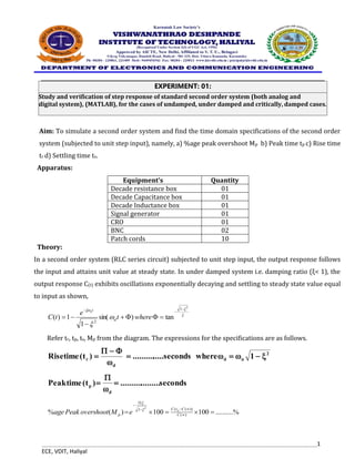
  • 1. 1 ECE, VDIT, Haliyal Aim: To simulate a second order system and find the time domain specifications of the second order system (subjected to unit step input), namely, a) %age peak overshoot Mp b) Peak time tp c) Rise time tr d) Settling time ts. Apparatus: Equipment’s Quantity Decade resistance box 01 Decade Capacitance box 01 Decade Inductance box 01 Signal generator 01 CRO 01 BNC 02 Patch cords 10 Theory: In a second order system (RLC series circuit) subjected to unit step input, the output response follows the input and attains unit value at steady state. In under damped system i.e. damping ratio (ξ< 1), the output response C(t) exhibits oscillations exponentially decaying and settling to steady state value equal to input as shown,      2 1 2 tan ) sin( 1 1 ) (           where t e t C d t n Refer tr, tp, ts, Mp from the diagram. The expressions for the specifications are as follows. 2 n d d r 1 where onds sec ..... .......... ) t ( time Rise            onds sec ......... .......... ) t ( time Peak d p     % .......... 100 100 ) ( % ) ( )) ( ( 1 2            C C t C p p e M overshoot Peak age   Study and verification of step response of standard second order system (both analog and digital system), (MATLAB), for the cases of undamped, under damped and critically, damped cases. EXPERIMENT: 01:
  • 2. 2 ECE, VDIT, Haliyal %) 2 ( onds sec ......... .......... 4 ) t ( time Settling %) 5 ( onds sec ......... .......... 3 ) t ( time Settling n s n s       L C 2 R ξ LC 1 ω (2) and (1) equation Comparing ) 2 ( 2 prototype order 2 Function Transfer ) 1 ( 1 1 ) ( ) ( V Function Transfer is function transfer the circuit, series RLC namely system order second a For n 2 2 2 nd 2 o                                      n n n i S S LC S L R S LC S V S    With increase in resistance, ξ increases where the oscillations are damped. At ξ = 1, the system is said to be critically damped, where the oscillations are completely damped out. For ξ >1, the system is said to be over-damped. For ξ=0, the system is said to undamped where sustained oscillations are produced. Procedure :- 1) Choose L=10mH, C=0.01uF arbitrarily. Calculate value of n & R for ξ=1 and ξ=1.5 respectively. Calculate theoretical values of tp,ts,tr,Mp with each case. 2) Apply a square wave input of 1 V (p-p) .Calibrate the CRO for time scale and amplitude scale. Adjust the resistance for ξ=0.2 i.e. under damped case. Note the corresponding response on CRO. Measure tp, tr, ts, Mp. Compare the measured quantities with the theoretical values, for verification. 3) Similarly adjust R for ξ=1, critically damped case. Note the corresponding response on CRO. Measure ts. 4) Also for ξ=0.5, adjust R correspondingly for Over damped case . Note the corresponding response on CRO. Measure only ts. 5) On graph sheet plot the response showing the quantities measured. Practically ξ=0, undamped case cannot be simulated as L & C elements have certain finite resistance.
  • 3. 3 ECE, VDIT, Haliyal Observations: - Sl. No R in Ω s Ξ tp in sec Tp sec Tr Sec Tr sec Ts sec Ts sec Mp in % age Mp in % age Actual Cal Actual Cal Actual Cal Actual Cal 01 200 0.1 02 2000 1.0 03 3000 1.5 Conclusion:- Write briefly about system response in each case of damping. Compare the settling times in each case. Calculations: The second order standard transfer function is given by. T. F = CIRCUIT DIAGRAM
  • 4. 4 ECE, VDIT, Haliyal MATLAB PROGRAM wn= input('frequency') zeta= input('damping factor') k= input('constant') num= [k*wn^2] deno= [1 2*zeta*wn wn^2] g= tf(num, deno) t= feedback(g,1) step(t, 'r') Example :
  • 5. 5 ECE, VDIT, Haliyal Aim:- To design a passive RC lead-lag compensating network for the specified maximum phase lead angle Фm and ωm, the frequency at which it occurs i.e. ωm and then determine it’s frequency Bode diagrams. Using the Bode diagrams, determine the transfer function of the lead compensating network Apparatus:- Equipments Quantity Decade resistance box 02 Decade Capacitance box 01 Signal generator 01 CRO 01 BNC 02 Patch cords 10 Theory:- Lead compensating network is used in control systems to stabilize unstable systems or to improve relative stability by improving gain margin and phase margin. Lead compensator used as series compensator has the following effects on the system performance. (Refer figure 1). a) Increase in bandwidth and speed of response. b) Decrease in maximum overshoot in response c) Improvement in relative stability with increase in PM. d) Acts as high pass filter attenuating low frequency signals and hence useful in low damped systems. To design a Lag-Lead compensator and to obtain the characteristics by simulation using MATLAB. Verify the performance using experiments with the compensator circuit made of passive elements EXPERIMENT: 02
  • 6. 6 ECE, VDIT, Haliyal Circuit Diagram : Characteristics: Design of passive RC lead compensating network From the specifications, it is desired to obtain maximum phase lead Фm =____________ at a frequency F=__________Hz ωm= 2ΠF=_________ rad/sec. 1. From 1 a 1 a sin m     , find ‘a’ substituting Фm. 2. From d m a 1    ,find Td substituting ωm and a.
  • 7. 7 ECE, VDIT, Haliyal 3. Assume C = 0.1μF 4. Determine R1 and R2. But, 2 2 1 d n n 2 1 2 2 1 2 1 d 1 n R R R a R R R ) R R /( C R R and C R              Design Calculations: for Φm=……….. degrees ωm=………..rad/sec. Procedure: 1. Rig up the designed lead compensating network as shown. 2. Using signal generator, apply sinusoidal input signal (about 2V p-p ) with the frequency varying over a wide range from 20 Hz to 300 kHz. 3. Increase the frequency of the input signal gradually and at each frequency note down peak to peak amplitude of input and output signals. Also note down the phase difference between the i/p and o/p signals using Lissageous pattern on CRO. 4. Maintain the amplitude of i/p signal constant at all frequencies. 5. Plot Bode’s magnitude and phase plots on semi log sheet. Observations: I/P signal (p-p) = 2V Frequency in Hz Input Voltage Vi Output Voltage Vo AB XY Gain in db = 20 log(Vo/Vi) Ф = sin (AB/XY)
  • 8. 8 ECE, VDIT, Haliyal Lissageous pattern MATLAB PROGRAM clc;close all;clear; %transfer function s=tf('s'); G=0.2/(s*(s+1)); %Root locus rlocus(G); %calculate the Shortage Phase syms s1 G1=0.2/(s1*(s1+1)); phi=double(angle(subs(G1,s1,-4+6.93i)))*180/pi; sphi=180-phi; %T , a z=-4; p=-4-6.93/tand(90-sphi); %shart andazeh Gc1=(s1-z)/(s1-p); kc=1/(double(abs(subs(Gc1*G1,-4+6.93i)))); %simulation Gc=(s-z)/(s-p); Gcloseloop=kc*Gc*G/(1+kc*Gc*G); figure; rlocus(Gc*G); Attach Printout of Program
  • 9. 9 ECE, VDIT, Haliyal EXPERIMENT: 03: Steady state error analysis for Type-0, Type-1, Type-2 digital control system using MATLAB by applying standard reference inputs of step , ramp and parabola. . A MATLAB program which will get the transfer function of the system and returns the following. a. System type as a string (Type 0 or Type 1 or Type 2) b. Steady state error for i. Step input ii. Ramp input iii. Parabolic input A system is called type 0, type 1, type 2,p , if N=0, N=1, N=2, p , respectively. Note that this classification is different from that of the order of a system. As the type number is increased, accuracy is improved; however, increasing the type number aggravates the stability problem. A compromise between steady-state accuracy and relative stability is always necessary. MATLAB PROGRAM clc; close all; clear all; h1=h2=h3=1; g1=zpk([-3 -5],[-7 -8],[1]); g2=zpk([-3 -5],[0 -7 -8],[1]); g3=zpk([-3 -5],[0 0 -7 -8],[1]); chk1=find(pole1==0); chk2=find(pole2==0); chk3=find(pole3==0); x1=length(chk1); x2=length(chk2); x3=length(chk3); fprintf('System 1 if of type %dn',x1); fprintf('System 2 if of type %dn',x2); fprintf('System 3 if of type %dn',x3); s=tf('s'); kp1=dcgain(g1*h1); kv1=dcgain(s*g1*h1); ka1=dcgain((s^2)*g1*h1); kp2=dcgain(g2*h2); kv2=dcgain(s*g2*h2); ka2=dcgain((s^2)*g2*h2); kp3=dcgain(g3*h3);
  • 11. 11 ECE, VDIT, Haliyal Design a digital controller with output feedback to control the speed of a DC motor; simulate the design using Simulink. EXPERIMENT: 04 AIM: To simulate a DC position control system using armature controlled DC motor in MATLAB and obtain its step response through state space approach for i) open loop ii) closed loop operations THEORY: a) Consider an armature controlled DC motor open loop position control system. From the state equations the state model is
  • 12. 12 ECE, VDIT, Haliyal From the state model Take KT = 1 Nm/Amp, Kb = 1 Volts/radians/sec, J = 4×10⁻³ Nm/radians/sec, Ra = 5Ώ, La = 1mH and f=2x10⁻³. Simulate the state space model in MATLAB to obtain its step response. % step response of open loop DC position control system f = 0.002; Kb = 1; La = 0.001; Ra = 5; KT = 1; Kb=1; J=4e-3; title (‘Step Response of open Loop DC position Control System’);
  • 13. 13 ECE, VDIT, Haliyal MATLAB PROGRAM t = 0:0.1:15; Td = -0.1 * (t>5 & t<10); % load disturbance u = [ones(size(t)) ; Td]; % w_ref=1 and Td cl_ff = dcm * diag([Kff,1]); % add feedforward gain cl_ff.InputName = {'w_ref','Td'}; cl_ff.OutputName = 'w'; h = lsimplot(cl_ff,u,t); title('Setpoint tracking and disturbance rejection') legend('cl_ff') % Annotate plot line([5,5],[.2,.3]); line([10,10],[.2,.3]); text(7.5,.25,{'disturbance','T_d = -0.1Nm'},... 'vertic','middle','horiz','center','color','r'); Expected Output
  • 14. 14 ECE, VDIT, Haliyal A linear model of the system can be extracted from the Simulink model into the MATLAB workspace. This can be accomplished employing the MATLAB command linmod or from directly within Simulink as we will do here. We will specifically use the base Simulink model developed from first principles shown below. You can download this model by right-clicking here and then selecting Save link as ..., or you can refer to the DC Motor Speed: Simulink Modeling page to recreate the model yourself. Recall that the physical parameters have to be set if they have not previously been defined in the workspace. J = 0.01; b = 0.1; K = 0.01; R = 1; L = 0.5; Design a digital controller with state variable feedback to control the speed of a DC motor; simulate the design using Simulink EXPERIMENT: 05
  • 15. 15 ECE, VDIT, Haliyal We then need to identify the inputs and outputs of the model we wish to extract. First right-click on the signal representing the Voltage input in the Simulink model. Then choose Linear Analysis Points > Open-loop Input from the resulting menu. Similarly, right-click on the signal representing the Speed output and select Linear Analysis Points > Open-loop Output from the resulting menu. The input and output signals should now be identified on your model by arrow symbols as shown in the figure below. In order to perform the extraction, select from the menus at the top of the model window Analysis > Control Design > Linear Analysis. This will cause the Linear Analysis Tool to open. Within the Linear Analysis Tool window, the Operating Point to be linearized about can remain the default, Model Initial Condition. In order to perform the linearization, next click the Step button identified by a step response with a small green triangle. The result of this linearization is the linsys1 object which will appear in the Linear Analysis Workspace as shown below. Furthermore, the open-loop step response of the linearized system also will be generated automatically. The open-loop step response above is consistent with the response generated in the DC Motor Speed: System Analysis page The reason the responses match so closely is because this Simulink model uses only linear components. Note that this process can be used to extract linear approximations of models with nonlinear elements too. We will further verify the model extraction by looking at the model itself. The linearized model can be exported by simply dragging the object into the MATLAB Workspace. This object can then be used within MATLAB in the same manner as an object created directly from the MATLAB command line. Specifically, entering the command zpk(linsys1) in the MATLAB command window demonstrates that the resulting model has the following form.(1)
  • 16. 16 ECE, VDIT, Haliyal This model matches the one generated in the DC Motor Speed: System Modeling page. This can be seen by repeating the MATLAB commands given below. s = tf('s'); P_motor = K/((J*s+b)*(L*s+R)+K^2); zpk(P_motor) ans = 2 ------------------- (s+9.997) (s+2.003) Open-loop response The open-loop step response can also be generated directly within Simulink, without extracting any models to the MATLAB workspace. In order to simulate the step response, the details of the simulation must first be set. This can be accomplished by selecting Model Configuration Parameters from the Simulation menu. Within the resulting menu, define the length for which the simulation is to run in the Stop time field. We will enter "3" since 3 seconds will be long enough for the step response to reach steady state. Within this window you can also specify various aspects of the numerical solver, but we will just use the default values for this example. Next we need to add an input signal and a means for displaying the output of our simulation. This is done by doing the following:  Remove the In1 and Out1 blocks.  Insert a Step block from the Simulink/Sources library and connect it with a line to the Voltage input of the motor subsystem.  To view the Speed output, insert a Scope from the Simulink/Sinks library and connect it to the Speed output of the motor subsystem.  To provide an appropriate unit step input at t=0, double-click the Step block and set the Step time to "0". The final model should appear as shown in the following figure. Then run the simulation (press Ctrl-T or select Run from the Simulation menu). When the simulation is finished, double-click on the scope and you should see the following output.
  • 17. 17 ECE, VDIT, Haliyal This response is identical to that obtained by MATLAB above using the extracted model. This is again to be expected because this Simulink model includes only linear blocks. Closed-loop response with lag compensator In the DC Motor Speed: Root Locus Controller Design page a lag compensator was designed with the following transfer function. (2) To generate the closed-loop step response with this compensator in Simulink, we will begin with the "Motor_Model.slx" file described above. We will then put the lag compensator in series with the motor subsystem and will feed back the motor's speed for comparison to a desired reference. More specifically, follow the steps given below:  Remove the Input and Output ports of the model.  Insert a Sum block from the Simulink/Math Operations library. Then double-click on the block and enter "|+-" for its List of signs where the symbol "|" serves as a spacer between ports of the block.  Insert a Transfer Function block from the Simulink/Continuous library. Then double-click on the block and edit the Numerator coefficients field to "[44 44]" and the Denominator coefficients field to "[1 0.01]".  Insert a Step block from the Simulink/Sources library. Then double-click on the block and set the Step time to "0".  Insert a Scope block from the Simulink/Sinks library. Then connect and label the components as shown in the following figure
  • 18. 18 ECE, VDIT, Haliyal You can download our version of the closed-loop system model by right-clicking here and then selecting Save link as .... Then run the simulation (press Ctrl-T or select Run from the Simulation menu). When the simulation is finished, double-click on the scope and you should see the following output. This step response matches exactly the closed-loop performance observed in the DC Motor Speed: Root Locus Controller Design page where the lag compensator was originally designed. Note that while we used the physics- based Simulink model developed in the DC Motor Speed: Simulink Modeling page for simulating the closed-loop system, we could have equivalently used the Simscape version of the DC motor model. Closed-loop response with lead compensator We have shown in the above and in other pages of this example that the lag compensator we have designed meets all of the given design requirements. Instead of a lag compensator, we could have also designed a lead compensator to meet the given requirements. More specifically, we could have designed a lead compensator to achieve a similar DC gain and phase margin to that achieved by the lag compensator, but with a larger gain crossover frequency. You can refer back to the DC Motor Speed: Frequency Domain Methods for Controller Design page for more details on
  • 19. 19 ECE, VDIT, Haliyal the design of the lag compensator, but the fact that the DC gains and phase margins are similar indicate that the responses under lag and lead control would have similar amounts of error in steady state and similar amounts of overshoot. The difference in response would come in that the larger gain crossover frequency provided by the lead compensator would make the system response faster than with the lag compensator. We will specifically use the following lead compensator.(3) To see the precise effect of the lead compensator as compared to our lag compensator, let's modify our Simulink model from above as follows:  Disconnect the Step block and Scope block from the rest of the model.  Copy the blocks forming the closed-loop of the model: the Sum block, the Transfer Function block, and the DC Motor subsystem. Then paste a copy of this loop below the original blocks.  Double-click on the Transfer Function block and edit the Numerator coefficients field to "[160000 5.6e6]" and the Denominator coefficients field to "[1 1035]".  Insert a Mux block from the SimulinkSignal Routing library and connect the outputs of the two Motor subsystem blocks to the inputs of the Mux and connect the output of the Mux to the Scope.  Connect the Step block to the Sum block of the original feedback system. Then branch off from this line and connect it to the Sum block of the lead compensated system as well. The Mux block serves to bundle the two signals into a single line, this way the Scope will plot both speed signals on the same set of axes. When you are done, your model should appear as follows. Running the simulation and observing the output produced by the scope, you will see that both responses have a steady-state error that approaches zero. Zooming in on the graphs you can generate a figure like the one shown below. Comparing the two graphs, the blue response belonging to the lead compensated system has a much smaller settle time and slightly larger, but similar, overshoot as compared to the yellow response produced by the lag compensated system.
  • 20. 20 ECE, VDIT, Haliyal It is generally preferred that a system respond to a command quickly. Why then might we prefer to use the lag compensator even though it is slower than the lead compensator? The advantage of the lag compensator in this case is that by responding more slowly it requires less control effort than the lead compensator. Less control effort means that less power is consumed and that the various components can be sized smaller since they do not have to supply as much energy or withstand the higher voltages and current required of the lead compensator. We will now modify our simulation to explicitly observe the control effort requirements of our two feedback systems. We will do this by sending our various signals to the workspace for plotting and further manipulation if desired. Specifically, delete the Scope and Mux blocks from your Simulink model. Then insert four To Workspace blocks from the SimulinkSinks library. Double-click on each of the blocks and change their Save format from Structure to Array. Also provide a Variable name within each block that will make sense to you. You can then connect the blocks to the existing model and label them as shown below. You can download our version of this Simulink model by right-clicking here and then selecting Save link as ....
  • 21. 21 ECE, VDIT, Haliyal Then change the simulation stop time to 1 second and run the model. The act of running the simulation will send to the MATLAB workspace a series of arrays corresponding to the variables set-up in your model with the To Workspace blocks. Furthermore, the time vector used by that run of the simulation is stored in the default variable tout. You can now plot the results of your simulation from the workspace. Enter the following code to see how to specifically plot the control effort variables. subplot(2,1,1) plot(tout,ulag); xlabel('time (seconds)') ylabel('control effort (volts)') title('Control Effort Under Lag Compensation') subplot(2,1,2) plot(tout,ulead); xlabel('time (seconds)') ylabel('control effort (volts)') title('Control Effort Under Lead Compensation')
  • 22. 22 ECE, VDIT, Haliyal This example shows how to use numerical optimization to tuning the controller parameters of a nonlinear system. In this example, we model a CE 152 Magnetic Levitation system where the controller is used to position a freely levitating ball in a magnetic field. The control structure for this model is fixed and the required controller performance can be specified in terms of an idealized time response. Earnshaw's Theorem Earnshaw's theorem proved that it is not possible to achieve stable levitation using static, macroscopic, classical electromagnetic fields. However the CE 152 system works around this by creating a potential well around the point at which the ball is to be suspended, thereby creating a non-inverse square law force. This is achieved by an inductive coil that generates a time varying electromagnetic field. The electromagnetic field is controlled through the use of feedback to keep the ball at the required location. open_system('maglev_demo') Design a digital controller with output feedback to control the position of the metallic ball in Magnetic levitation experiment and simulate the design using Simulink EXPERIMENT: 06
  • 23. 23 ECE, VDIT, Haliyal Model Description The magnetic levitation system is a nonlinear dynamic system with one input and one output. Double-click the Magnetic Levitation Plant Model to open this subsystem. The input voltage is applied to a coil that creates the electromagnetic field. The output voltage is measured by an IR receiver and represents the position of the ball in the magnetic field. The diagram below outlines this system. The physical system consists of a ball (with mass 0.00837 kg) which is under the influence of three forces:  The magnetic field produced by an inductive coil. This is modeled by the Power amplifier and coil block in the Simulink® model. The input to the inductor is a voltage signal and the output a current. The force from the coil depends on the square of the current, the air-gap between the coil and the ball, and the physical properties of the ball. This produces an upward acting force on the ball.  The gravitational force acting downwards  A damping force which acts in a direction opposite to the velocity at any instant of time These three forces cause the resulting motion of the ball and are modeled in Simulink as shown. open_system('maglev_demo/Magnetic Levitation Plant Model')
  • 24. 24 ECE, VDIT, Haliyal Non-linearities arising from saturation of the coil and changes in dynamics outside the limits of the magnetic field are also modeled in the Simulink Model. As the force from the coil decays according to an inverse square law larger voltages are required the further the ball is from the coil. The control signal is scaled to account for this and the scaling is included in the Control signal scaling blocks. Control Problem Description The requirement for the controller is that it be able to position the ball at any arbitrary location in the magnetic field and that it move the ball from one position to another. These requirements are captured by placing step response bounds on the position measurement. Specifically we require the following constraints on the ball:  Position constraint: within 20% of the desired position in less than 0.5 second  Settling Time Constraint: within 2% of the desired position within 1.5 second To meet the control requirements we implement a Proportional-Integral-Derivative (PID) controller. For convenience the controller uses a normalized position measurement with a range from 0 to 1, representing the bottom-most and top-most positions of the ball respectively. Simulink® Design Optimization™ and numerical optimization is ideally suited to tune the PID coefficients because:  The system dynamics are complex enough to require effort and time for analysis if we approach the problem using conventional control design techniques.  The controller structure is fixed.  We have knowledge of the step response we require from the system. Setting Constraint Values Given the step response characteristic we desire, it is simple to specify the upper and lower bounds of the response. Double-click the Position Constraint block in the Magnetic Levitation Plant Model subsystem to view constraints on the position of the ball. The constraint lines may be moved using the mouse.
  • 25. 25 ECE, VDIT, Haliyal You can launch the Response Optimizer using the Apps menu in the Simulink toolstrip, or the sdotool command in MATLAB®. You can launch a pre-configured optimization task in the Response Optimizer by first opening the model and by double-clicking on the orange block at the bottom of the model. From the Response Optimizer, press the Plot Model Response button to simulate the model and show how well the initial design satisfies the design requirements. Defining Tuned Parameters
  • 26. 26 ECE, VDIT, Haliyal We select the PID controller parameters to tune by opening the Design Variables editor, as shown below. Running the Optimization After specifying the optimization parameters and the required step response bounds we start the optimization by pressing the Optimize button from the Response Optimizer. During optimization, the plots are updated with the position of the ball for each iteration and the dark curve shows the final optimized trajectory of the ball (as shown below).
  • 27. 27 ECE, VDIT, Haliyal Verifying the Results Once we complete the optimization, it is important to validate the results against other step sizes. A successful parameter optimization should be able to provide good control for all steps sizes close to the tuned step size of 1. Step sizes from .7 to 1 should be tested to confirm the controller's performance. The following plot shows the response to a step input from 0 to 0.85 at 0.1 seconds. Conclusion The verification step shows that controller's performance satisfies the requirements specified and the tuned parameter values are suitable for control. The tuned parameters could be used to provide baseline performance against which other control schemes can be compared, or a baseline for controllers for different operating regions. % Close the model. bdclose('maglev_demo')
  • 28. 28 ECE, VDIT, Haliyal Equipment needed  Arduino board (e.g. Uno, Mega 2560, etc.)  lightbulb (incandescent, LED, CFL, etc.)  AC solid-state relay (hockey-puck type, etc.)  temperature sensor (TMP36, etc.) The temperature of the lightbulb is measured in this example with a TMP36 sensor (cheap, relatively accurate, sufficient range). The Arduino board provides power to the sensor and reads the sensor output via an Analog Input. The Arduino board is also used for generating the Digital Output that switches the solid-state relay on and off. That is, the digital output alternately connects and disconnects the light bulb from the AC power source (from the wall) via the relay in order to turn the light bulb on and off. The control logic employed for determining when to switch the relay on and off is implemented within Simulink, which is also employed for visualizing the light bulb's temperature and the control signal. System identification experiment In order to implement our temperature control system, we technically don't need a model of our plant (the light bulb). We can simply employ logic that turns the light bulb on when the measured temperature is lower than desired and turns the light bulb off when the temperature is higher than desired. We, however, would like to be able to explain the resulting behavior of our control system (and perhaps even attempt to design the control algorithm in a more intelligent manner). Therefore, we will generate a model for the thermal behavior of the light bulb based on its observed response. This is sometimes referred to as a blackbox model or a data-driven model. After we have generated such a model, we will attempt to explain what we have observed based on our understanding of the underlying physics. Hardware setup In this experiment our plant is a standard incandescent light bulb where we will (ultimately) attempt to control the light bulb's temperature. We have chosen a 25 W bulb in order to keep the maximum temperature within the limits of the temperature sensor we have chosen. You can also employ other types of bulbs (LED, CFL, etc.). For our temperature sensor, we will employ the TMP36 (though many others can be employed). This sensor measures temperature in Celsius, is quite inexpensive (a couple of dollars), has adequate range, reasonable accuracy, and doesn't need to be calibrated. This sensor is also commonly included in many Arduino starter kits that are in the market place. The datasheet for this sensor can be found here. The temperature sensor can be attached to the surface of the lightbulb employing thermally conductive epoxy, or with adhesive metal tape. The TMP36 is connected to the Arduino Board as shown below. Specifically, if the sensor is oriented such that the pins are pointed downward and the flat side of the sensor is facing you, then the leftmost pin is the power (must be between 2.7 V and 5.5 V), the middle pin is the signal, and the rightmost pin is ground. Power and ground for the TMP36 are supplied from the Arduino board and the signal, which is a voltage that is linearly proportional to temperature, is read on one of the board's Analog Inputs. Implement an on-off temperature controller to control lamp using a temperature sensor and dspace DS1104 hardware interface EXPERIMENT: 07
  • 29. 29 ECE, VDIT, Haliyal The lightbulb is turned on and off employing a digital output from the Arduino board via a solid-state relay. The solid-state relay is basically an electrical switch that can connect/disconnect a (possibly high-power) device to an AC source with a low-power DC signal. In our case, the AC source comes from a standard wall outlet and the DC signal is supplied by a Digital Output from our Arduino board. Therefore, our solid-state relay needs to be able to handle 120-240 V on the AC side (in North America need 120 V) and the DC side must be able to be controlled with a 5 V signal. Since our load (the lightbulb) is resistive (not inductive) and doesn't require much current, we don't have to be very particular about the solid-state relay we employ. We are in particular employing a simple "hockey-puck" style relay. In order to control the lightbulb, we need to insert the relay into the circuit (the loop) that connects the lightbulb to the wall. Therefore, we must cut into the cord for the lightbulb and wire the relay into the circuit. In doing this, make sure that the bulb is not plugged in. You should insert the relay on the neutral wire of the bulb's plug. The neutral wire is indicated by a white stripe or ribbing. If you insert the relay on the live wire, then the terminals of the relay are connected to the power supply even when the relay is off. You should also cover the exposed terminals of the relay and never touch the terminals when the bulb is plugged in.
  • 30. 30 ECE, VDIT, Haliyal MAT LAB PROGRAM s = tf('s'); To = 18.5; % ambient/initial temperature K = 83.5; % DC gain tau = 66; % time constant P = K/(tau*s+1); % model transfer function [y,t] = step(P,350); % model step response plot(t+50,y+To); hold plot(temp,'r:') xlabel('time (sec)') ylabel('temperature (degrees C)') title('Lightbulb Temperature Step Response') legend('model','experiment','Location','SouthEast') EXPECTED OUTPUT
  • 31. 31 ECE, VDIT, Haliyal Equipment needed  Arduino board (e.g. Uno, Mega 2560, etc.)  lightbulb (incandescent, LED, CFL, etc.)  AC solid-state relay (hockey-puck type, etc.)  temperature sensor (TMP36, etc.) The temperature of the lightbulb is measured in this example with a TMP36 sensor (cheap, relatively accurate, sufficient range). The Arduino board provides power to the sensor and reads the sensor output via an Analog Input. The Arduino board is also used for generating the Digital Output that switches the solid-state relay on and off. That is, the digital output alternately connects and disconnects the light bulb from the AC power source (from the wall) via the relay in order to turn the light bulb on and off. The control logic employed for determining when to switch the relay on and off is implemented within Simulink, which is also employed for visualizing the light bulb's temperature and the control signal. System identification experiment In order to implement our temperature control system, we technically don't need a model of our plant (the light bulb). We can simply employ logic that turns the light bulb on when the measured temperature is lower than desired and turns the light bulb off when the temperature is higher than desired. We, however, would like to be able to explain the resulting behavior of our control system (and perhaps even attempt to design the control algorithm in a more intelligent manner). Therefore, we will generate a model for the thermal behavior of the light bulb based on its observed response. This is sometimes referred to as a blackbox model or a data-driven model. After we have generated such a model, we will attempt to explain what we have observed based on our understanding of the underlying physics. Hardware setup In this experiment our plant is a standard incandescent light bulb where we will (ultimately) attempt to control the light bulb's temperature. We have chosen a 25 W bulb in order to keep the maximum temperature within the limits of the temperature sensor we have chosen. You can also employ other types of bulbs (LED, CFL, etc.). For our temperature sensor, we will employ the TMP36 (though many others can be employed). This sensor measures temperature in Celsius, is quite inexpensive (a couple of dollars), has adequate range, reasonable accuracy, and doesn't need to be calibrated. This sensor is also commonly included in many Arduino starter kits that are in the market place. The datasheet for this sensor can be found here. The temperature sensor can be attached to the surface of the lightbulb employing thermally conductive epoxy, or with adhesive metal tape. The TMP36 is connected to the Arduino Board as shown below. Specifically, if the sensor is oriented such that the pins are pointed downward and the flat side of the sensor is facing you, then the leftmost pin is the power (must be between 2.7 V and 5.5 V), the middle pin is the signal, and the rightmost pin is ground. Power and ground for the TMP36 are supplied from the Arduino board and the signal, which is a voltage that is linearly proportional to temperature, is read on one of the board's Analog Inputs. The lightbulb is turned on and off employing a digital output from the Arduino board via a solid-state relay. The solid-state relay is basically an electrical switch that can connect/disconnect a (possibly high-power) device to an Design a digital controller with output feedback to control the speed of a DC motor; Control the DC motor using dspace DS1104 hardware interface EXPERIMENT: 08
  • 32. 32 ECE, VDIT, Haliyal AC source with a low-power DC signal. In our case, the AC source comes from a standard wall outlet and the DC signal is supplied by a Digital Output from our Arduino board. Therefore, our solid-state relay needs to be able to handle 120-240 V on the AC side (in North America need 120 V) and the DC side must be able to be controlled with a 5 V signal. Since our load (the lightbulb) is resistive (not inductive) and doesn't require much current, we don't have to be very particular about the solid-state relay we employ. We are in particular employing a simple "hockey-puck" style relay. In order to control the lightbulb, we need to insert the relay into the circuit (the loop) that connects the lightbulb to the wall. Therefore, we must cut into the cord for the lightbulb and wire the relay into the circuit. In doing this, make sure that the bulb is not plugged in. You should insert the relay on the neutral wire of the bulb's plug. The neutral wire is indicated by a white stripe or ribbing. If you insert the relay on the live wire, then the terminals of the relay are connected to the power supply even when the relay is off. You should also cover the exposed terminals of the relay and never touch the terminals when the bulb is plugged in.
  • 33. 33 ECE, VDIT, Haliyal MAT LAB PROGRAM s = tf('s'); To = 18.5; % ambient/initial temperature K = 83.5; % DC gain tau = 66; % time constant P = K/(tau*s+1); % model transfer function [y,t] = step(P,350); % model step response plot(t+50,y+To); hold plot(temp,'r:') xlabel('time (sec)') ylabel('temperature (degrees C)') title('Lightbulb Temperature Step Response') legend('model','experiment','Location','SouthEast') EXPECTED OUTPUT