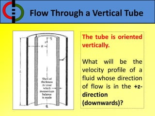
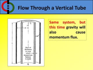
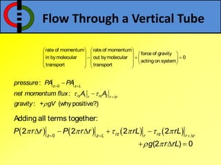
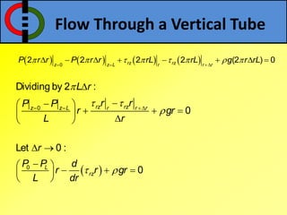
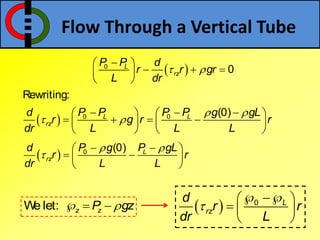
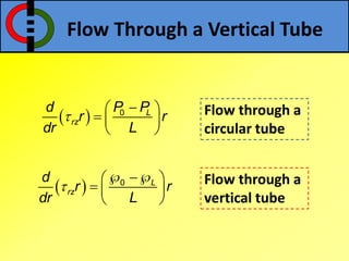
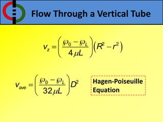
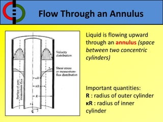
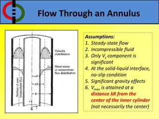
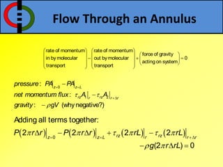
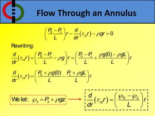
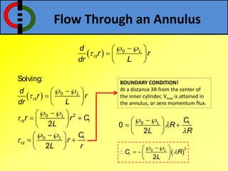
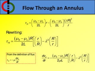
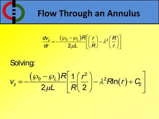
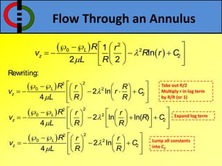
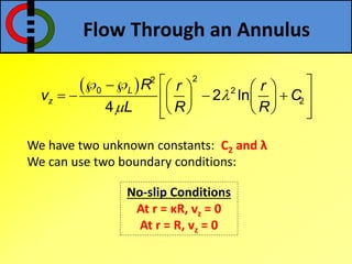
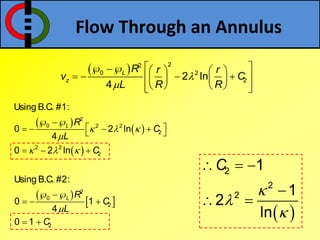
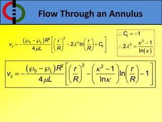
This document outlines flow through a vertical tube and an annulus. For a vertical tube, the momentum equation is developed showing that the velocity profile is parabolic. Gravity causes a downward acceleration. For an annulus, assumptions are made and the momentum equation is similarly developed. It is shown that the maximum velocity occurs at a distance λ from the inner cylinder and that the velocity profile takes a logarithmic form.

1. Shell Momentum Balances

2. Outline
1.Flow Through a Vertical Tube
2.Flow Through an Annulus
3.Exercises

3. Flow Through a Vertical Tube
The tube is oriented
vertically.
What will be the
velocity profile of a
fluid whose direction
of flow is in the +z-
direction
(downwards)?

4. Flow Through a Vertical Tube
Same system, but
this time gravity will
also cause
momentum flux.

5. Flow Through a Vertical Tube
rate of momentum rate of momentum
force of gravity
in by molecular out by molecular 0
acting on system
transport transport
   
    
      
    
   
0
1 2
:
:
: + (whypositive?)
z z L
rz rzr r r
pressure PA PA
net momentum flux A A
gravity gV
 

 



       0
Adding all terms together:
2 2 2 2
(2 ) 0
rz rzz z L r r r
P r r P r r rL rL
g r rL
     
 
  
    
  

6. Flow Through a Vertical Tube
 
0
0
Dividing by 2 :
0
Let 0 :
0
rz rzz z L r r r
L
rz
L r
r rP P
r gr
L r
r
P P d
r r gr
L dr

 

 
  

 
   
 
 
     
 
       0
2 2 2 2 (2 ) 0rz rzz z L r r r
P r r P r r rL rL g r rL         
       

7. Flow Through a Vertical Tube
 0
0L
rz
P P d
r r gr
L dr
 
 
   
 
  0 0
Rewriting:
(0)L L
rz
d P P P P g gL
r g r r
dr L L L
 
 
     
      
   
We let: z zP gz     0 L
rz
d
r r
dr L

  
  
 
  0 (0) L
rz
d P g P gL
r r
dr L L
 

  
  
 

8. Flow Through a Vertical Tube
  0 L
rz
d
r r
dr L

  
  
 
  0 L
rz
d P P
r r
dr L

 
  
 
Flow through a
circular tube
Flow through a
vertical tube

9. Flow Through a Vertical Tube
 2 20
4
L
zv R r
L
  
  
 
20
32
L
avev D
L
  
  
 
Hagen-Poiseuille
Equation

10. Outline
1.Flow Through a Vertical Tube
2.Flow Through an Annulus
3.Exercises

11. Flow Through an Annulus
Liquid is flowing upward
through an annulus (space
between two concentric
cylinders)
Important quantities:
R : radius of outer cylinder
κR : radius of inner
cylinder

12. Flow Through an Annulus
Assumptions:
1. Steady-state flow
2. Incompressible fluid
3. Only Vz component is
significant
4. At the solid-liquid interface,
no-slip condition
5. Significant gravity effects
6. Vmax is attained at a
distance λR from the
center of the inner cylinder
(not necessarily the center)

13. Flow Through an Annulus
rate of momentum rate of momentum
force of gravity
in by molecular out by molecular 0
acting on system
transport transport
   
    
      
    
   
0
1 2
:
:
: (whynegative?)
z z L
rz rzr r r
pressure PA PA
net momentum flux A A
gravity gV
 

 




       0
Adding all terms together:
2 2 2 2
(2 ) 0
rz rzz z L r r r
P r r P r r rL rL
g r rL
     
 
  
    
  

14. Flow Through an Annulus
 0
0L
rz
P P d
r r gr
L dr
 
 
   
 
  0 0
Rewriting:
(0)L L
rz
d P P P P g gL
r g r r
dr L L L
 
 
     
      
   
We let: z zP gz     0 L
rz
d
r r
dr L

  
  
 
  0 (0) L
rz
d P g P gL
r r
dr L L
 

  
  
 

15. Flow Through an Annulus
  0 L
rz
d
r r
dr L

  
  
 
  0
20
1
0 1
Solving:
2
2
L
rz
L
rz
L
rz
d
r r
dr L
r r C
L
C
r
L r



  
  
 
  
  
 
  
  
 
BOUNDARY CONDITION!
At a distance λR from the center of
the inner cylinder, Vmax is attained in
the annulus, or zero momentum flux.
0 1
0
2
L C
R
L R


  
  
 
 
20
1
2
L
C R
L

  
   
 

16. Flow Through an Annulus
 0 2
Rewriting:
2
L
rz
R r R
L R r
 
      
     
    
 
2
0 0
2 2
L L
rz
R
r
L L r


      
    
   
From the definition of flux:
z
rz
dv
dr
  
 0 2
2
Lz
Rdv r R
dr L R r


      
      
    

17. Flow Through an Annulus
 0 2
2
Lz
Rdv r R
dr L R r


      
      
    
 
 
2
0 2
2
Solving:
1
ln
2 2
L
z
R r
v R r C
L R


    
     
  

18. Flow Through an Annulus
 
 
2
0 2
2
1
ln
2 2
L
z
R r
v R r C
L R


    
     
  
  22
0 2
2
Rewriting:
2 ln
4
L
z
R r R
v r C
L R R


      
        
     
Take out R/2
Multiply r in log term
by R/R (or 1)
Expand log term
Lump all constants
into C2
  22
0 2
22 ln ln( )
4
L
z
R r r
v R C
L R R


       
         
      
  22
0 2
22 ln
4
L
z
R r r
v C
L R R


      
       
     

19. Flow Through an Annulus
  22
0 2
22 ln
4
L
z
R r r
v C
L R R


      
       
     
We have two unknown constants: C2 and λ
We can use two boundary conditions:
No-slip Conditions
At r = κR, vz = 0
At r = R, vz = 0

20. Flow Through an Annulus
  22
0 2
22 ln
4
L
z
R r r
v C
L R R


      
       
     
 
 
 
2
0 2 2
2
2 2
2
Using B.C. #1:
0 2 ln
4
0 2 ln
L R
C
L
C
  

  
 
     
  
 
2
2
2
1
1
2
ln
C



  

  
 
2
0
2
2
Using B.C. #2:
0 1
4
0 1
L R
C
L
C

 
  
 

21. Flow Through an Annulus
  22
0 2
22 ln
4
L
z
R r r
v C
L R R


      
       
       
2
2
2
1
1
2
ln
C



  

 
  22 2
0 1
ln 1
4 ln
L
z
R r r
v
L R R

 
       
        
      

22. Shell Balances
1. Identify all the forces that influence the flow
(pressure, gravity, momentum flux) and their
directions. Set the positive directions of your axes.
2. Create a shell with a differential thickness across the
direction of the flux that will represent the flow
system.
3. Identify the areas (cross-sectional and surface areas)
and volumes for which the flow occurs.
4. Formulate the shell balance equation and the
corresponding differential equation for the
momentum flux.

23. Shell Balances
5. Identify all boundary conditions (solid-liquid, liquid-
liquid, liquid-free surface, momentum flux values at
boundaries, symmetry for zero flux).
6. Integrate the DE for your momentum flux and
determine the values of the constants using the BCs.
7. Insert Newton’s law (momentum flux definition) to
get the differential equation for velocity.
8. Integrate the DE for velocity and determine values of
constants using the BCs.
9. Characterize the flow using this velocity profile.

24. Shell Balances
Important Assumptions*
1. The flow is always assumed to be at steady-
state.
2. Neglect entrance and exit effects. The flow is
always assumed to be fully-developed.
3. The fluid is always assumed to be
incompressible.
4. Consider the flow to be unidirectional.
*unless otherwise stated

25. Design Equations for Laminar
and Turbulent Flow in Pipes

26. Outline
1.Velocity Profiles in Pipes
2.Pressure Drop and Friction Loss (Laminar
Flow)
3.Friction Loss (Turbulent Flow)
4.Frictional Losses in Piping Systems

27. Velocity Profiles in Pipes
Recall velocity profile in a circular tube:
1. What is the shape of this profile?
2. The maximum occurs at which region?
3. What is the average velocity of the fluid
flowing through this pipe?
 2 20
4
L
z
P P
v R r
L
 
  
 

28. Velocity Profiles in Pipes

29. Velocity Profiles in Pipes
Velocity Profile in a Pipe:
Average Velocity of a Fluid in a Pipe:
 2 20
4
L
z
P P
v R r
L
 
  
 
20
32
L
ave
P P
v D
L
 
  
 

30. Maximum vs. Average Velocity

31. Outline
1.Velocity Profiles in Pipes
2.Pressure Drop and Friction Loss (Laminar
Flow)
3.Friction Loss (Turbulent Flow)
4.Frictional Losses in Piping Systems

32. Recall: Hagen-Poiseuille
Equation
20
32
L
ave
P P
v D
L
 
  
 
Describes the pressure drop and flow of
fluid (in the laminar regime) across a
conduit with length L and diameter D

33. Hagen-Poiseuille Equation
0 2
32 ave
L
Lv
P P
D

 
Pressure drop / Pressure loss (P0 – PL):
Pressure lost due to skin friction

34. Friction Loss
0 2
32 ave
L
Lv
P P
D

 
In terms of energy
lost per unit mass: 2
32O L ave
f
P P Lv
F
D

 

 
Mechanical energy lost due to friction in
pipe (because of what?)

35. Friction Factor
Definition: Drag force per wetted surface
unit area (or shear stress at the surface)
divided by the product of density times
velocity head
 
 
 
0
2 2
2 2
L C SS
P P A A
f
v v

 
   

36. Friction Factor
2
4
2
f
F
c c
F L v
f
g D g

Frictional force/loss head is proportional
to the velocity head of the flow and to
the ratio of the length to the diameter of
the flow stream

37. Friction Factor for Laminar Flow
Consider the Hagen-Poiseuille equation
(describes laminar flow) and the
definition of the friction factor:
Prove:
20
32
L
ave
P P
v D
L
 
  
 
2
4
2
f O L
F
c c
F P P L v
f
g g D g

 
Re
16
Ff
N
 Valid only for laminar flow

38. Outline
1.Velocity Profiles in Pipes
2.Pressure Drop and Friction Loss (Laminar
Flow)
3.Friction Loss (Turbulent Flow)
4.Frictional Losses in Piping Systems

39. Friction Factor for Turbulent
Flow
1. Friction factor is dependent on NRe and
the relative roughness of the pipe.
2. The value of fF is determined
empirically.
2
4
2
f
F
c c
F L v
f
g D g


40. Friction Factor for Turbulent
Flow
How to compute/find the value of the friction factor for
turbulent flow:
1. Use Moody diagrams.
- Friction factor vs. Reynolds number with a series of
parametric curves related to the relative roughness
2. Use correlations that involve the friction factor f.
- Blasius equation, Colebrook formula, Churchill
equation (Perry 8th Edition)

41. Moody Diagrams
Important notes:
1. Both fF and NRe are plotted in logarithmic scales.
Some Moody diagrams show fD (Darcy friction
factor). Make the necessary conversions.
2. No curves are shown for the transition region.
3. Lowest possible friction factor for a given NRe in
turbulent flow is shown by the smooth pipe line.

44. 1. Blasius equation for turbulent flow in smooth
tubes:
2. Colebrook formula
0.25
Re
0.079
Ff
N
 5
Re4000 10N 
10
Re
1 2.51
2log
3.7D D
Df N f
 
   
 
 
Friction Factor Correlations

45. 3. Churchill equation (Colebrook formula explicit in fD)
4. Swamee-Jain correlation
0.9
10
Re
1 0.27 7
2log
D
D Nf
  
         
10 0.9
Re
0.25
5.74
2log
3.7
Df
D N


 
 
 
Friction Factor Correlations

46. Materials of Construction Equivalent Roughness (m)
Copper, brass, lead (tubing) 1.5 E-06
Commercial or welded steel 4.6 E-05
Wrought iron 4.6 E-05
Ductile iron – coated 1.2 E-04
Ductile iron – uncoated 2.4 E-04
Concrete 1.2 E-04
Riveted Steel 1.8 E-03
Equivalent Roughness, ε

47. Instead of deriving new correlations for f, an approximation
is developed for an equivalent diameter, Deq, which may be
used to calculate NRe and f.
where RH = hydraulic radius
S = cross-sectional area
Pw = wetted perimeter: sum of the length
of the boundaries of the cross-section
actually in contact with the fluid
4 4eq H
w
S
D R
P
 
Frictional Losses for Non-Circular
Conduits

48. Determine the equivalent diameter of the
following conduit types:
1. Annular space with outside diameter Do and
inside diameter Di
2. Rectangular duct with sides a and b
3. Open channels with liquid depth y and liquid
width b
4 4eq H
w
S
D R
P
 
Equivalent Diameter (Deq)