This document contains diagrams and equations related to fluid mechanics concepts such as:
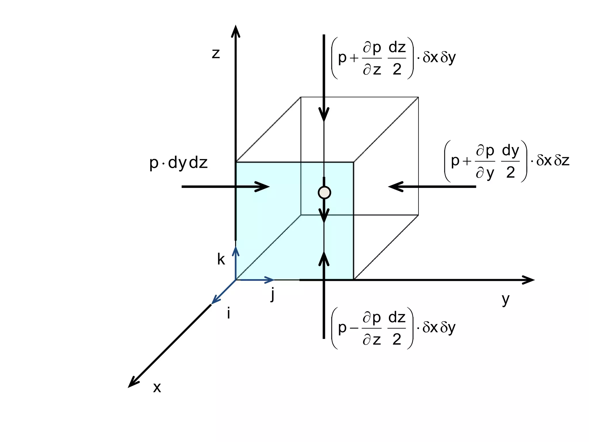
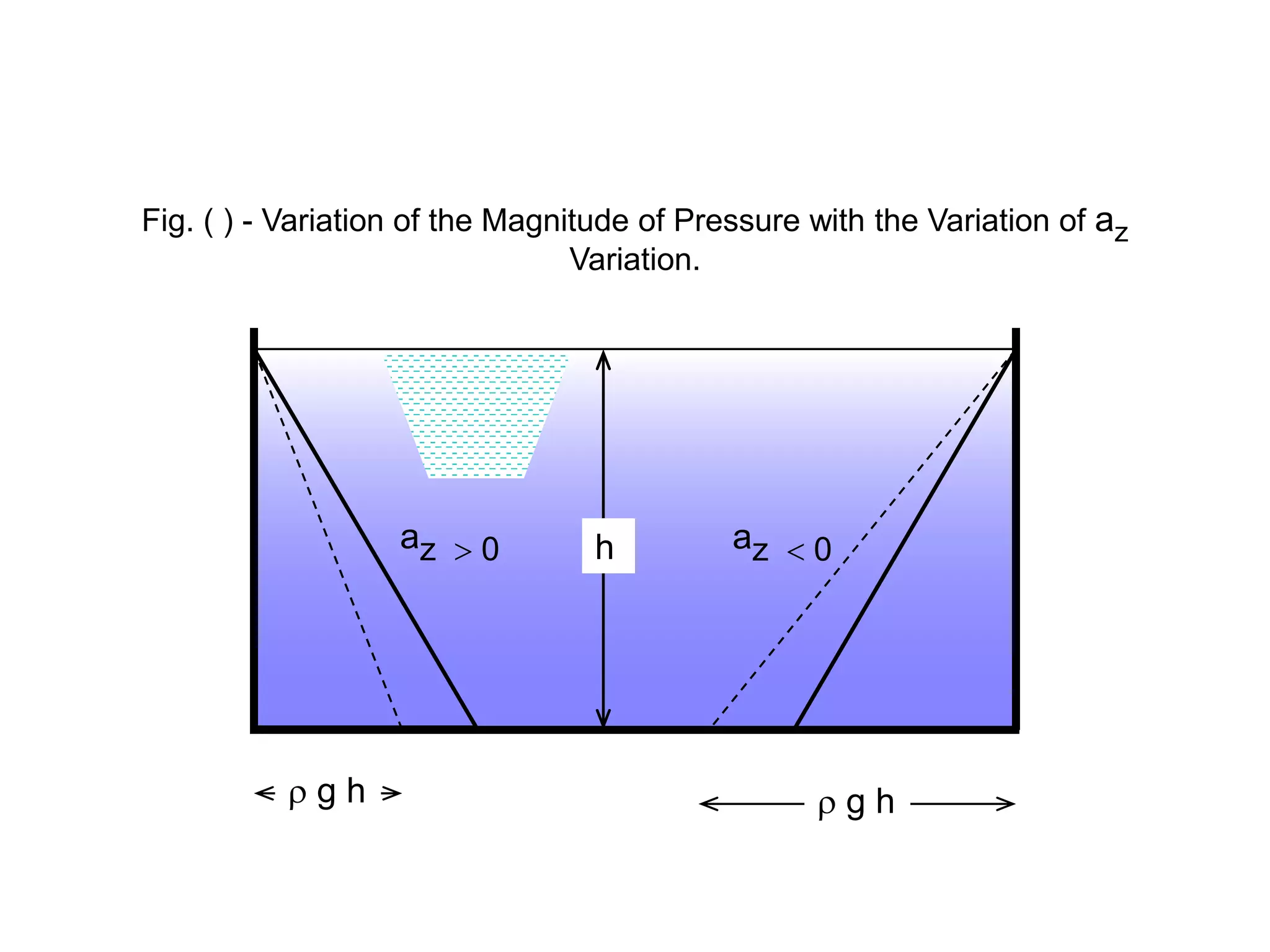
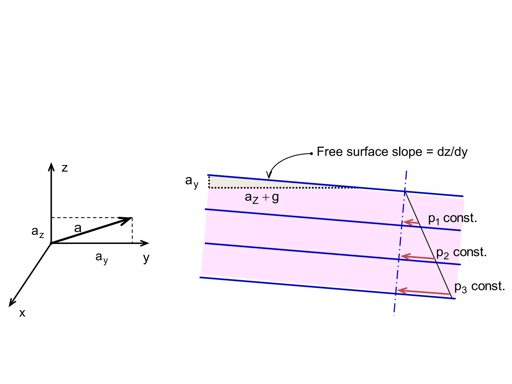
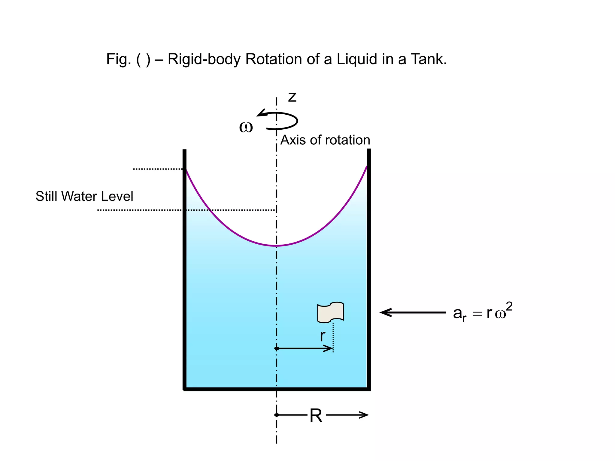
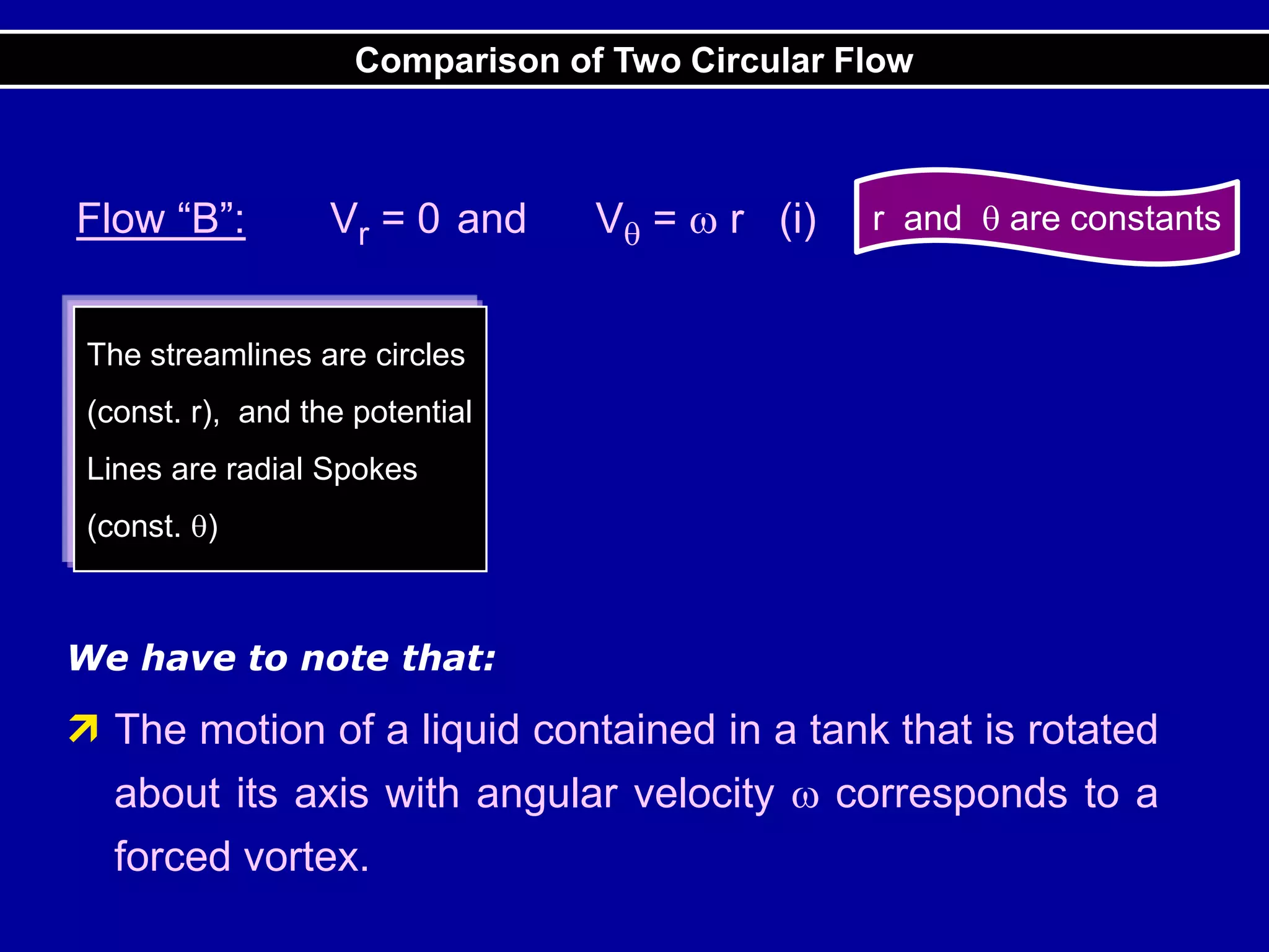
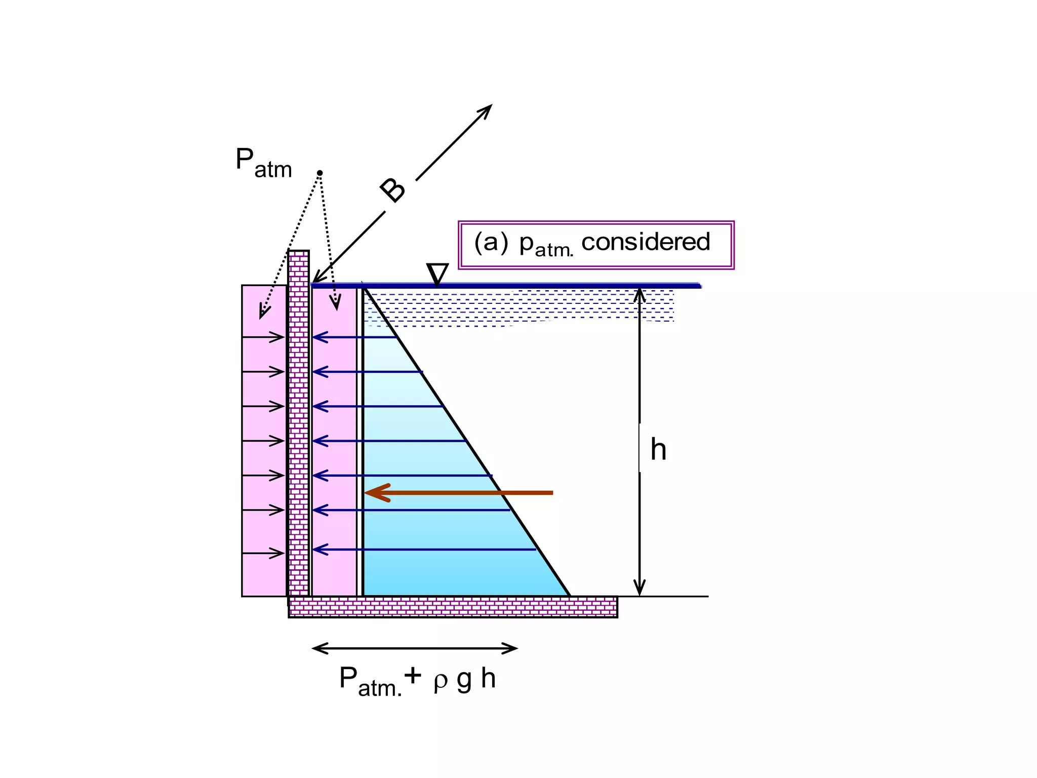
- Pressure variations in fluids undergoing acceleration or rigid body rotation
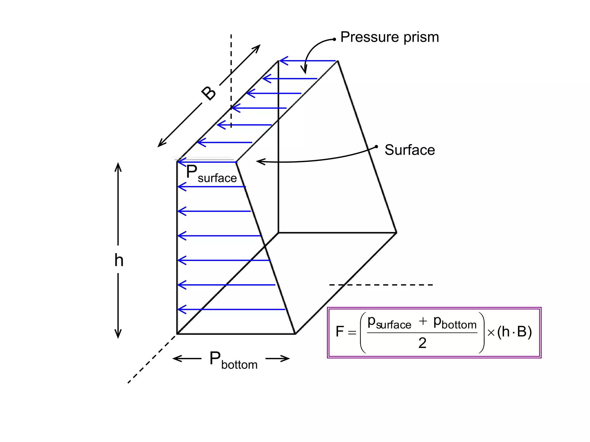
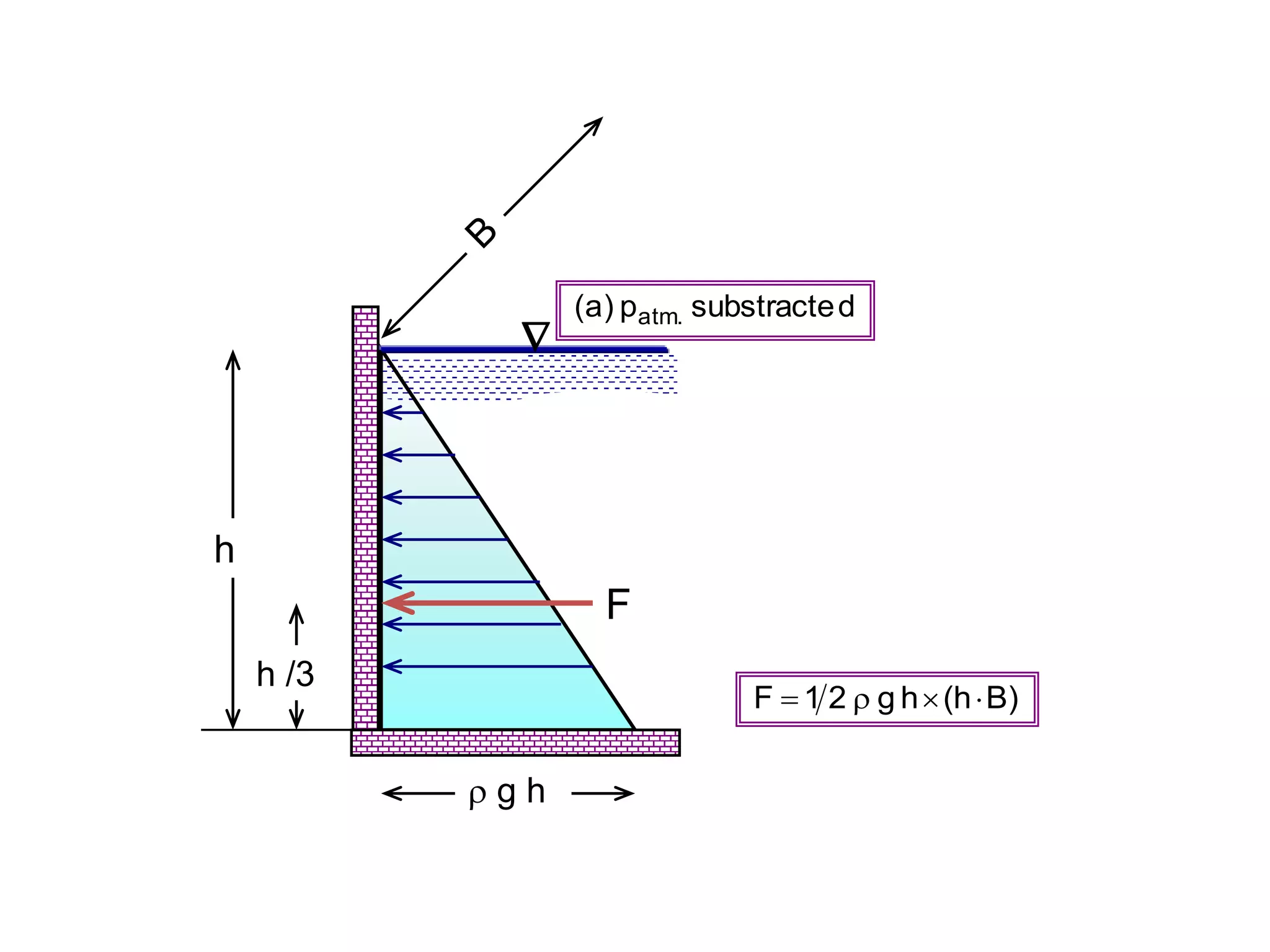
- Free surface profiles and pressure distributions in fluids in rotating or accelerated containers
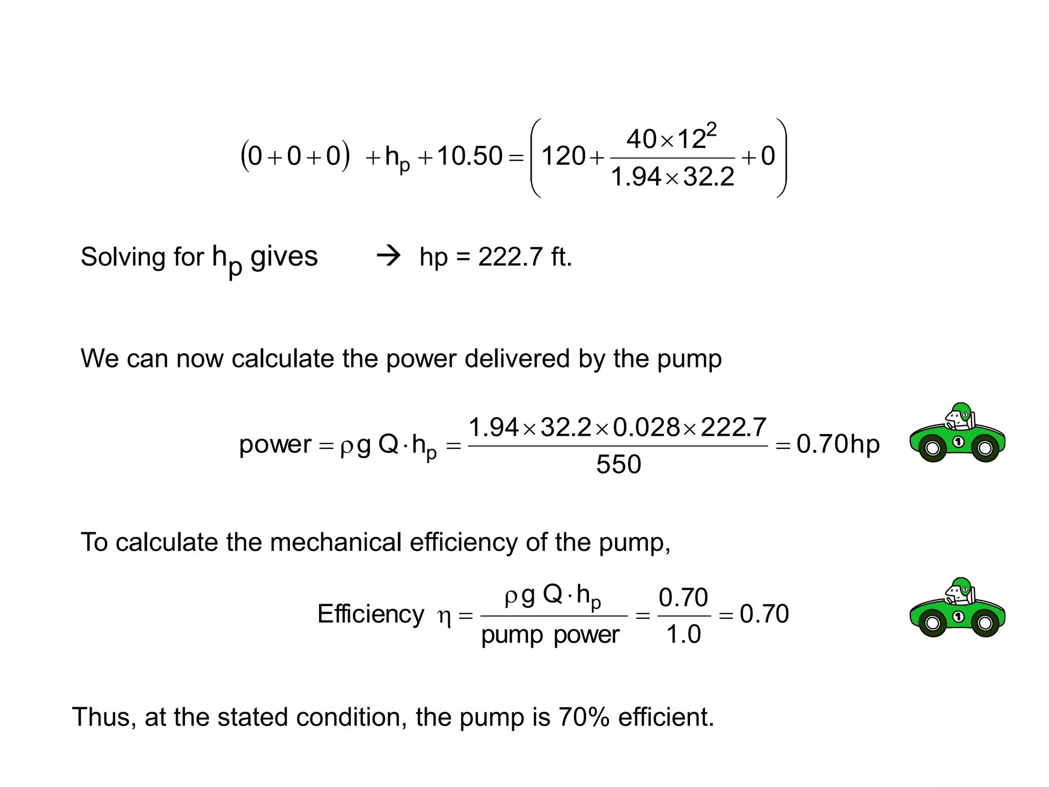
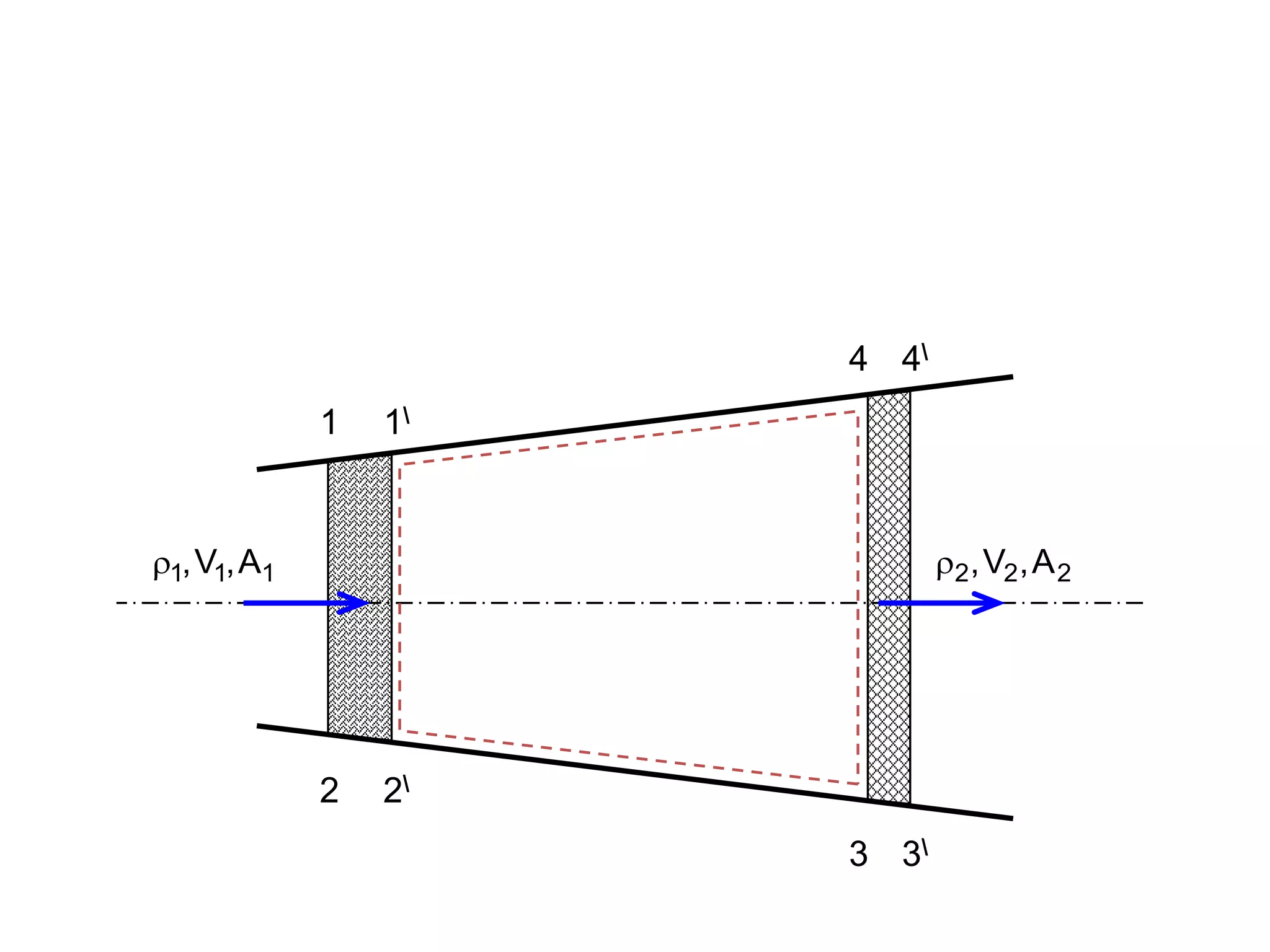
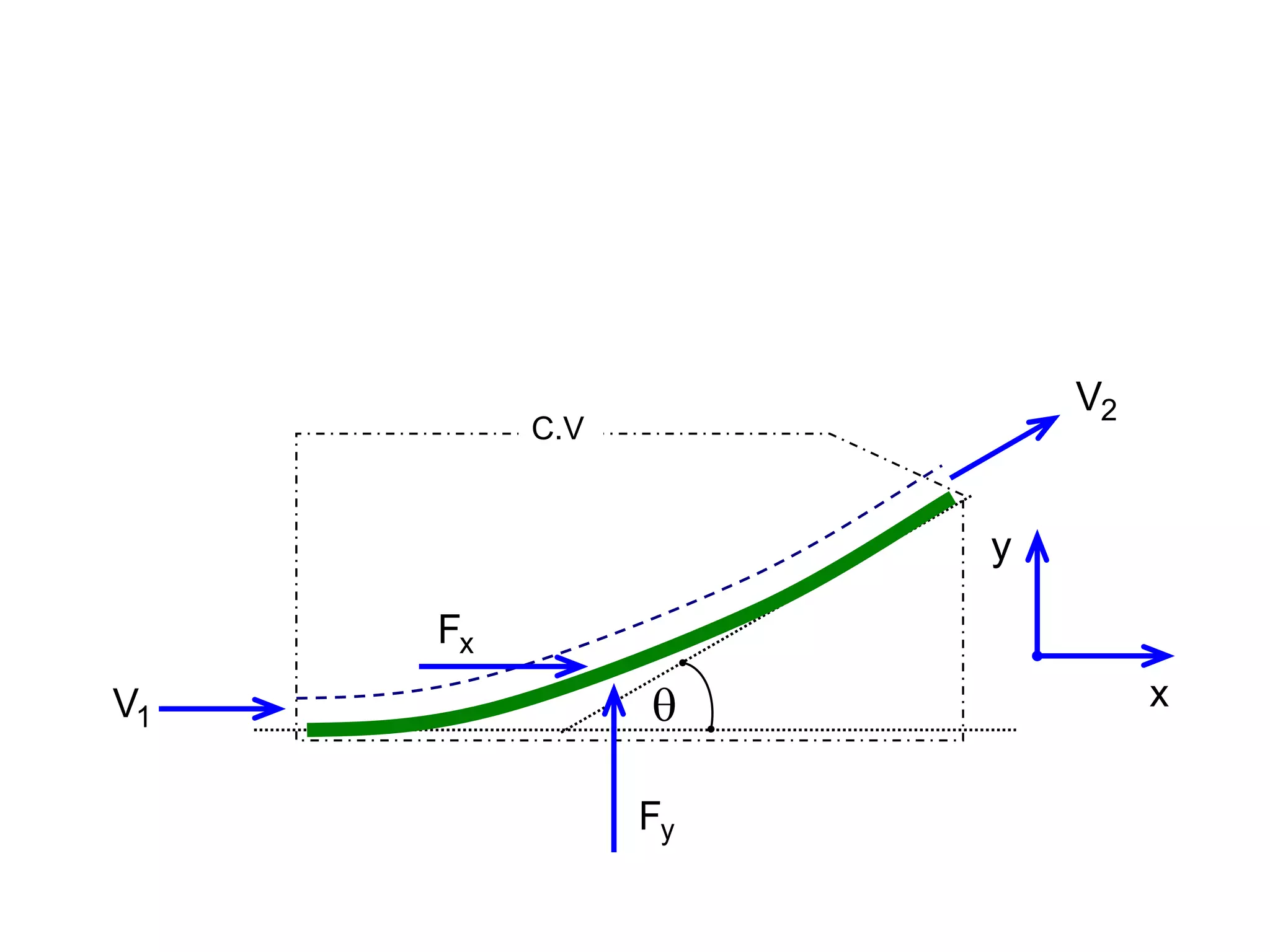
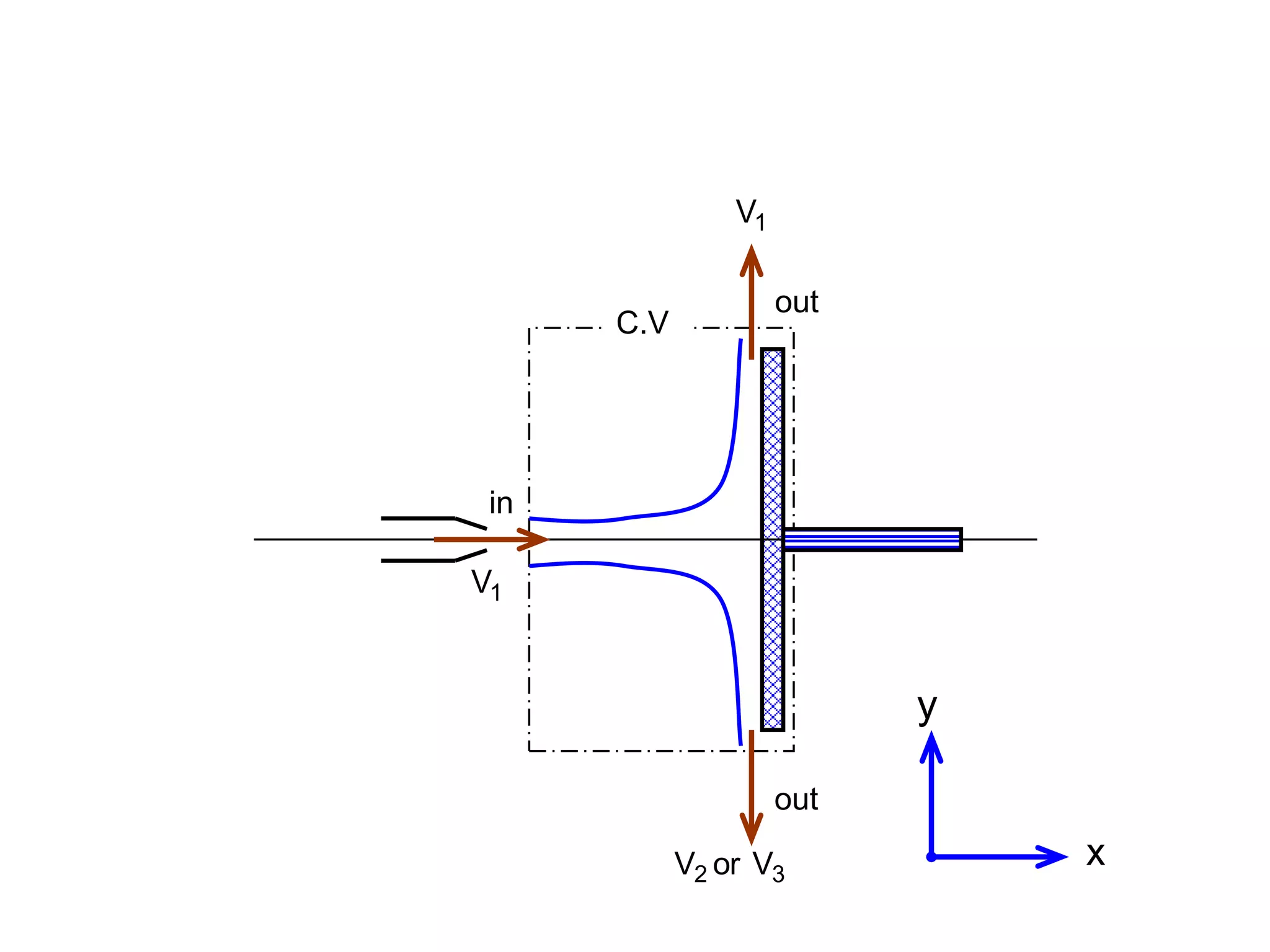
- Equations relating pressure, depth, acceleration/rotation, and density for both static and dynamic fluid situations