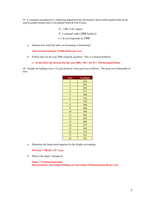
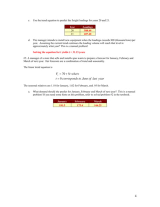
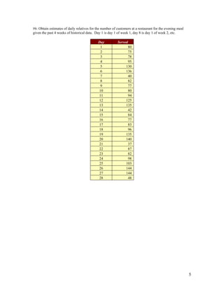
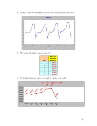
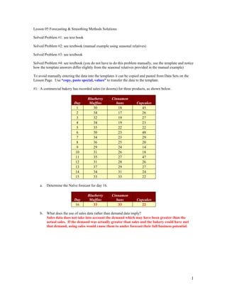
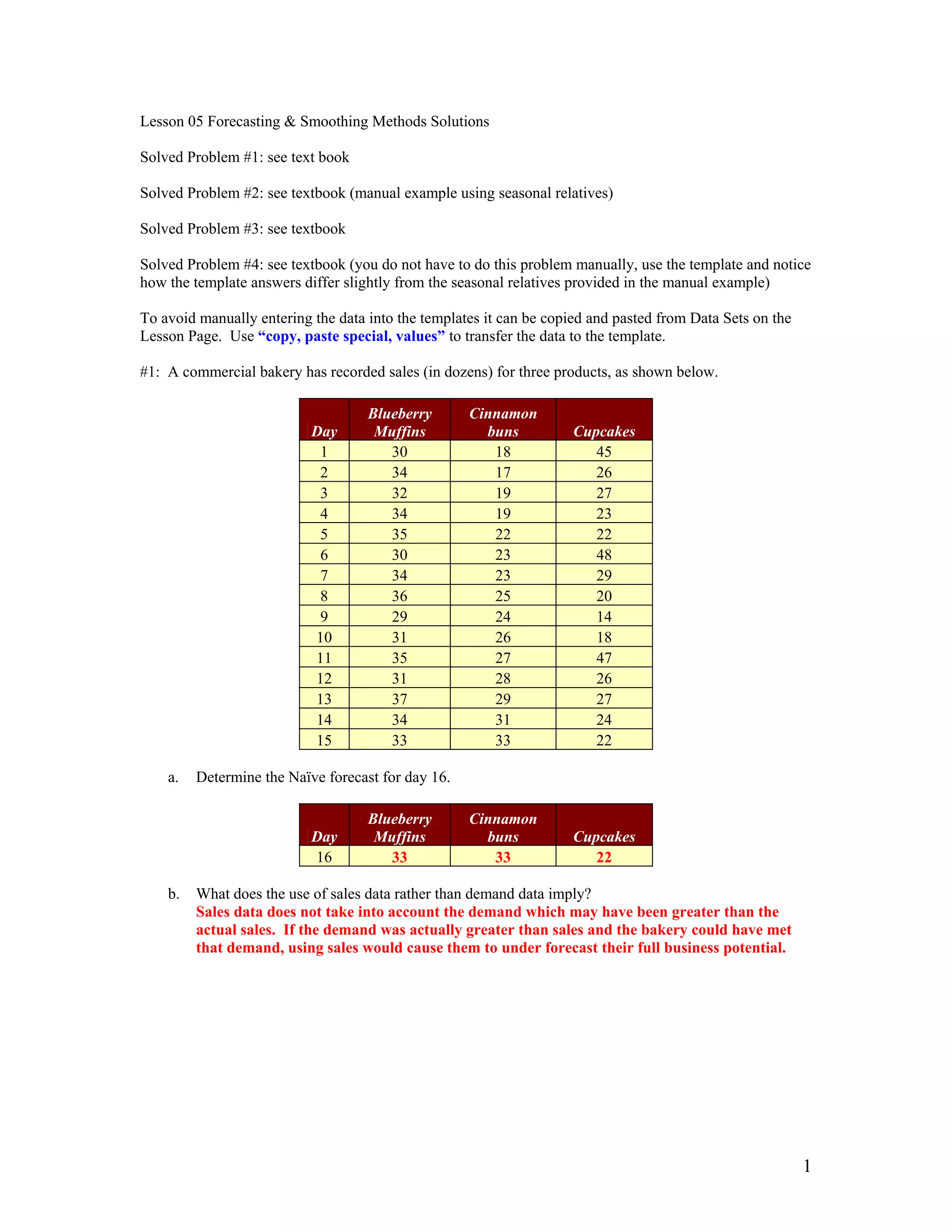
This document contains instructions and examples for 7 problems involving forecasting and smoothing methods. It includes instructions to copy data from external sources into templates to solve forecasting problems. The problems cover a variety of forecasting techniques including naive, moving averages, exponential smoothing, and trend analysis. Seasonal adjustment is demonstrated through examples calculating seasonal relatives for sales, customers, grain shipments and other time-series data. Forecasts are generated and compared to historical data for evaluation.

1. Lesson 05 Forecasting & Smoothing Methods Solutions
Solved Problem #1: see text book
Solved Problem #2: see textbook (manual example using seasonal relatives)
Solved Problem #3: see textbook
Solved Problem #4: see textbook (you do not have to do this problem manually, use the template and notice
how the template answers differ slightly from the seasonal relatives provided in the manual example)
To avoid manually entering the data into the templates it can be copied and pasted from Data Sets on the
Lesson Page. Use “copy, paste special, values” to transfer the data to the template.
#1: A commercial bakery has recorded sales (in dozens) for three products, as shown below.
Day
Blueberry
Muffins
Cinnamon
buns Cupcakes
1 30 18 45
2 34 17 26
3 32 19 27
4 34 19 23
5 35 22 22
6 30 23 48
7 34 23 29
8 36 25 20
9 29 24 14
10 31 26 18
11 35 27 47
12 31 28 26
13 37 29 27
14 34 31 24
15 33 33 22
a. Determine the Naïve forecast for day 16.
Day
Blueberry
Muffins
Cinnamon
buns Cupcakes
16 33 33 22
b. What does the use of sales data rather than demand data imply?
Sales data does not take into account the demand which may have been greater than the
actual sales. If the demand was actually greater than sales and the bakery could have met
that demand, using sales would cause them to under forecast their full business potential.
1

2. #2: National Scan, Inc., sells radio frequency inventory tags. Monthly sales ($000) for a seven-month
period were as follows:
Month Sales
Feb 19
Mar 18
Apr 15
May 20
Jun 18
Jul 22
Aug 20
a. Plot the monthly data.
Historical Data
0
5
10
15
20
25
0 1 2 3 4 5 6 7
Period
8
Sales
b. Forecast September sales volume in thousands of dollars using the following methods: Show your
answers in the space provided.
1. Naïve
2. Five-month moving average
3. Weighted moving average using .60 for August, .30 for July, and .10 for June
4. Exponential smoothing with a smoothing constant of .20
5. Linear trend equation.
Month Naive MA WMA ES LT
Sep 20 19 20.4 19.26 20.86
2

3. #3: A cosmetics manufacturer’s marketing department has developed a linear trend equation that can be
used to predict annual sales of its popular Hand & Foot Cream.
19900
)000(
1580
toscorrespondt
bottlessalesannualF
wheretF
t
t
=
=
+=
a. Indicate how much the sales are increasing or decreasing?
Sales are increasing by 15,000 bottles per year
b. Predict sales for the year 2006 using the equation? This is a manual problem!
t = 16 therefore the forecast for the year 2006 = 80 + 16*15 = 320 thousand bottles
#4: Freight car loadings over a 12-year period at a busy port are as follows: The units are in thousands of
tons.
Year Loadings
1 220
2 245
3 280
4 275
5 300
6 310
7 350
8 360
9 400
10 380
11 420
12 450
13 460
14 475
15 500
16 510
17 525
18 541
a. Determine the linear trend equation for the freight car loadings.
Forecast = 208.48 + 19 * year
b. What is the slope? Interpret it.
Slope = 19 thousand pounds
Interpretation: the freight loadings are increasing 19 thousand pounds per year
3

4. c. Use the trend equation to predict the freight loadings for years 20 and 21.
Year Loadings
20 588.40
21 607.40
d. The manager intends to install new equipment when the loadings exceeds 800 (thousand tons) per
year. Assuming the current trend continues the loading volume will reach that level in
approximately what year? This is a manual problem!
Solving the equation for t yields t = 31.13 years
#5: A manager of a store that sells and installs spas wants to prepare a forecast for January, February and
March of next year. Her forecasts are a combination of trend and seasonality.
The linear trend equation is
yearlastofJunetoscorrespondt
wheretFt
0
570
=
+=
The seasonal relatives are 1.10 for January, 1.02 for February, and .95 for March.
a. What demand should she predict for January, February and March of next year? This is a manual
problem! If you need some hints on this problem, refer to solved problem #2 in the textbook.
January February March
181.5 173.4 166.25
4

5. #6: Obtain estimates of daily relatives for the number of customers at a restaurant for the evening meal
given the past 4 weeks of historical data. Day 1 is day 1 of week 1, day 8 is day 1 of week 2, etc.
Day Served
1 80
2 75
3 78
4 95
5 130
6 136
7 40
8 82
9 77
10 80
11 94
12 125
13 135
14 42
15 84
16 77
17 83
18 96
19 135
20 140
21 37
22 87
23 82
24 98
25 103
26 144
27 144
28 48
5

6. a. Construct a graph that will enable you to visualize the daily variation in meals served.
Historical Data
0
20
40
60
80
100
120
140
160
0 5 10 15 20 25 30
Period
Served
b. What are the daily adjusted seasonal relatives?
Day
Adjusted
Seasonal
Relative
1 0.8997
2 0.8334
3 0.9160
4 1.0312
5 1.4116
6 1.4825
7 0.4256
c. Plot the adjusted seasonal relatives on a graph for each day of the week?
Adjusted Seasonal Relative (ASR)
0.8997
0.8334
0.9160
1.0312
1.411
0.0000
0.2000
0.4000
0.6000
0.8000
1.0000
1.2000
1.4000
1.6000
Period 1 Period
2
Period
3
Period
4
Period
5
Period
6
Period
7
6
1.4825
0.4256
6

7. d. Determine the forecast for meals to be served for the next 7 days.
Day Forecast
1 91.36
2 85.05
3 93.95
4 106.30
5 146.23
6 154.33
7 44.53
e. Plot historical demand with forecast on the same graph.
Historical Data & Seasonally Adjusted Linear Trend
0
20
40
60
80
100
120
140
160
180
0 10 20 30 40 50 60 70
Served Forecast
#7: A farming cooperative manager wants to estimate quarterly relatives for grain shipments, based on the
5 years of data shown below (quantities are in metric tons). You will have to enter this data into the
template manually.
QUARTER
Year 1 2 3 4
1 200 250 210 340
2 210 252 212 360
3 215 260 220 358
4 225 272 233 372
5 232 284 240 381
7

8. a. Calculate the quarterly adjusted seasonal relatives.
Quarter
Adjusted
Seasonal
Relative
1 0.8262
2 0.9919
3 0.8321
4 1.3499
b. Use the adjusted seasonal relative to determine what percentage shipments in quarter 4 are greater
than shipments quarter 3.
Quarter 4 shipments are 62.23% greater than shipments in quarter 3.
8