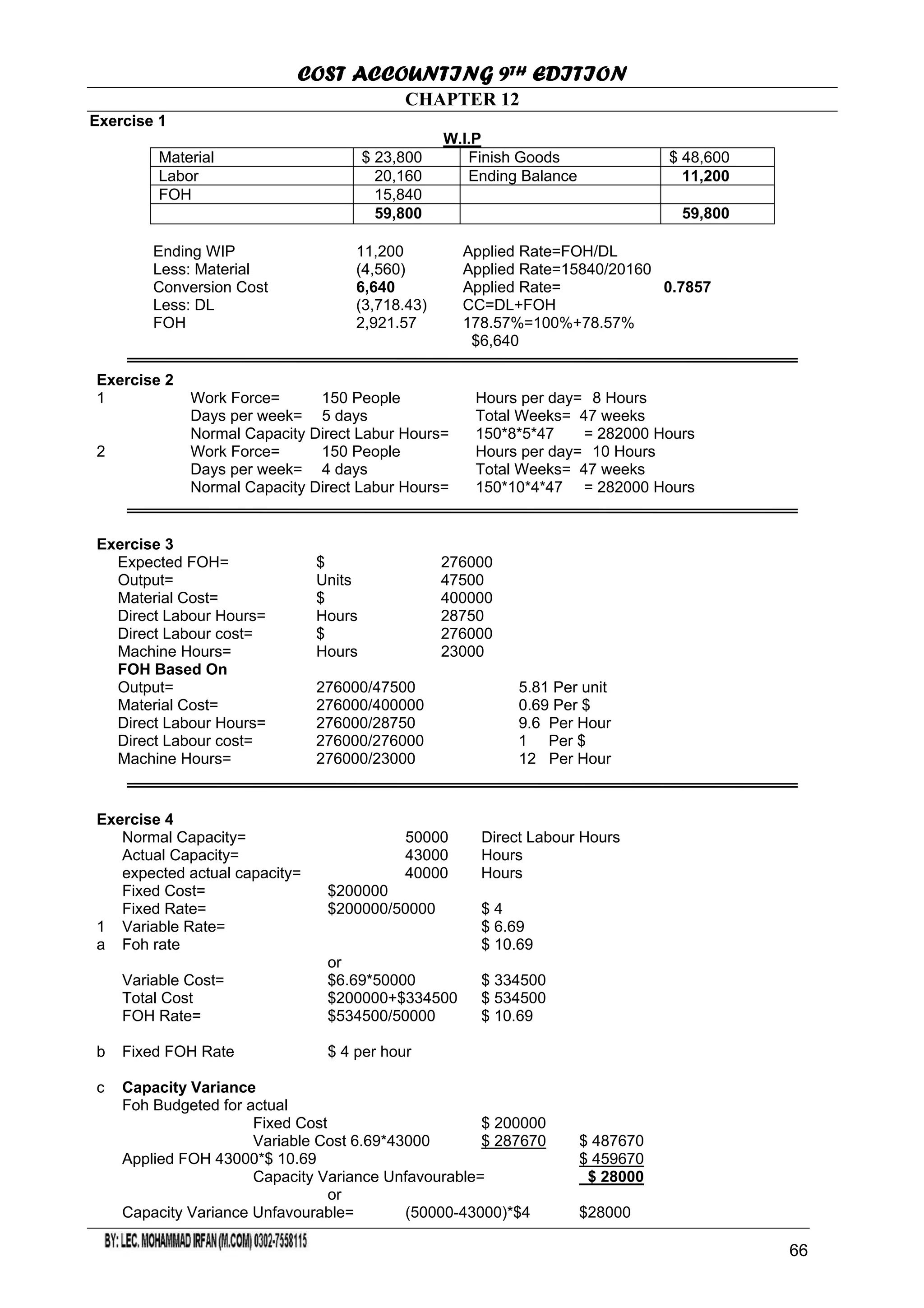
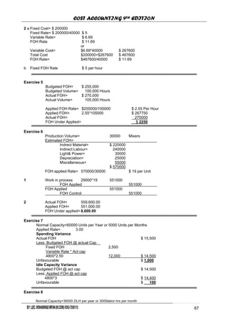
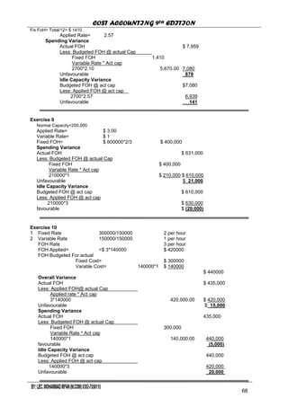
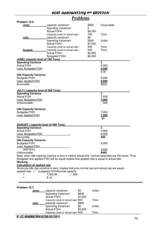
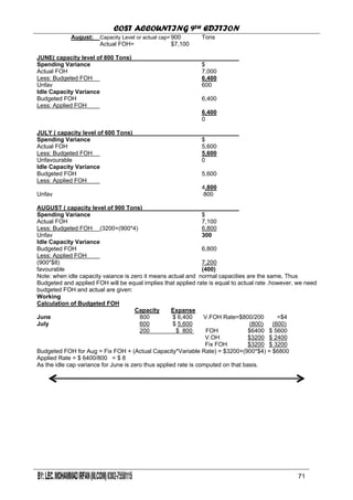
This document summarizes exercises from Chapter 12 of Cost Accounting, 9th Edition. It includes 11 exercises covering topics like work-in-process, overhead application rates, fixed and variable overhead rates, normal and actual capacity, budgeted and actual overhead, and overhead variances including spending and idle capacity variances. Calculations are shown for overhead application, budgeting, and analyzing variances at different production capacity levels.

1. COST ACCOUNTING 9TH EDITION
Chapter 12 Page 67
CHAPTER 12
Exercise 1
W.I.P
Ending WIP 11,200 Applied Rate=FOH/DL
Less: Material (4,560) Applied Rate=15840/20160
Conversion Cost 6,640 Applied Rate= 0.7857
Less: DL (3,718.43) CC=DL+FOH
FOH 2,921.57 178.57%=100%+78.57%
$6,640
Exercise 2
1 Work Force= 150 People Hours per day= 8 Hours
Days per week= 5 days Total Weeks= 47 weeks
Normal Capacity Direct Labur Hours= 150*8*5*47 = 282000 Hours
2 Work Force= 150 People Hours per day= 10 Hours
Days per week= 4 days Total Weeks= 47 weeks
Normal Capacity Direct Labur Hours= 150*10*4*47 = 282000 Hours
Exercise 3
Expected FOH= $ 276000
Output= Units 47500
Material Cost= $ 400000
Direct Labour Hours= Hours 28750
Direct Labour cost= $ 276000
Machine Hours= Hours 23000
FOH Based On
Output= 276000/47500 5.81 Per unit
Material Cost= 276000/400000 0.69 Per $
Direct Labour Hours= 276000/28750 9.6 Per Hour
Direct Labour cost= 276000/276000 1 Per $
Machine Hours= 276000/23000 12 Per Hour
Material $ 23,800 Finish Goods $ 48,600
Labor 20,160 Ending Balance 11,200
FOH 15,840
59,800 59,800
Exercise 4
Normal Capacity= 50000 Direct Labour Hours
Actual Capacity= 43000 Hours
expected actual capacity= 40000 Hours
Fixed Cost= $200000
Fixed Rate= $200000/50000 $ 4
1 Variable Rate= $ 6.69
a Foh rate $ 10.69
or
Variable Cost= $6.69*50000 $ 334500
Total Cost $200000+$334500 $ 534500
FOH Rate= $534500/50000 $ 10.69
b Fixed FOH Rate $ 4 per hour
c Capacity Variance
Foh Budgeted for actual
Fixed Cost $ 200000
Variable Cost 6.69*43000 $ 287670 $ 487670
Applied FOH 43000*$ 10.69 $ 459670
Capacity Variance Unfavourable= $ 28000
or
Capacity Variance Unfavourable= (50000-43000)*$4 $28000
61
66

2. COST ACCOUNTING 9TH EDITION
Chapter 12 Page 68
2 a Fixed Cost= $ 200000
Fixed Rate= $ 200000/40000 $ 5
Variable Rate= $ 6.69
FOH Rate $ 11.69
or
Variable Cost= $6.69*40000 $ 267600
Total Cost $200000+$267600 $ 467600
FOH Rate= $467600/40000 $ 11.69
b Fixed FOH Rate $ 5 per hour
Exercise 5
Budgeted FOH= $ 255,000
Budgeted Volume= 100,000 Hours
Actual FOH= $ 270,000
Actual Volume= 105,000 Hours
Applied FOH Rate= $255000/100000 $ 2.55 Per Hour
Applied FOH= 2.55*105000 $ 267750
Actual FOH= 270000
FOH Under Applied= $ 2250
Exercise 6
Production Volume= 30000 Mixers
Estimated FOH=
Indrect Material= $ 220000
Indirect Labour= 240000
Light& Power= 30000
Depreciation= 25000
Miscellaneous= 55000
$ 570000
FOH applied Rate= 570000/30000 $ 19 per Unit
1 Work in process 29000*19 551000
FOH Applied 551000
FOH Applied 551000
FOH Control 551000
2 Actual FOH= 559,600.00
Applied FOH= 551,000.00
FOH Under applied=8,600.00
Exercise 7
Normal Capacity=60000 Units per Year or 5000 Units per Months
Applied Rate= 3.00
Spending Variance
Actual FOH $ 15,500
Less: Budgeted FOH @ actual Cap
Fixed FOH 2,500
Variable Rate * Act cap
4800*2.50 12,000 $ 14,500
Unfavourable $ 1,000
Idle Capacity Variance
Budgeted FOH @ act cap $ 14,500
Less: Applied FOH @ act cap
4800*3 $ 14,400
Unfavourable $ 100
Exercise 8
Normal Capacity=36000 DLH per year or 3000labor hrs per month
6267

3. COST ACCOUNTING 9TH EDITION
Chapter 12 Page 69
Fix FoH= Total/12= $ 1410
Applied Rate= 2.57
Spending Variance
Actual FOH $ 7,959
Less: Budgeted FOH @ actual Cap
Fixed FOH 1,410
Variable Rate * Act cap
2700*2.10 5,670.00 7,080
Unfavourable 879
Idle Capacity Variance
Budgeted FOH @ act cap $7,080
Less: Applied FOH @ act cap
2700*2.57 6,939
Unfavourable 141
Exercise 9
Normal Capacity=200,000
Applied Rate= $ 3.00
Variable Rate= $ 1
Fixed FOH= $ 600000*2/3 $ 400,000
Spending Variance
Actual FOH $ 631,000
Less: Budgeted FOH @ actual Cap
Fixed FOH $ 400,000
Variable Rate * Act cap
210000*1 $ 210,000 $ 610,000
Unfavourable $ 21,000
Idle Capacity Variance
Budgeted FOH @ act cap $ 610,000
Less: Applied FOH @ act cap
210000*3 $ 630,000
favourable $ (20,000)
Exercise 10
1 Fixed Rate 300000/150000 2 per hour
2 Variable Rate 150000/150000 1 per hour
FOH Rate 3 per hour
FOH Applied= =$ 3*140000 $ 420000
FOH Budgeted For actual
Fixed Cost= $ 300000
Varable Cost= 140000*1 $ 140000
$ 440000
Overall Variance
Actual FOH $ 435,000
Less: Applied FOH@ actual Cap
Applied rate * Act cap
3*140000 420,000.00 $ 420,000
Unfavourable $ 15,000
Spending Variance
Actual FOH 435,000
Less: Budgeted FOH @ actual Cap
Fixed FOH 300,000
Variable Rate * Act cap
140000*1 140,000.00 440,000
favourable (5,000)
Idle Capacity Variance
Budgeted FOH @ act cap 440,000
Less: Applied FOH @ act cap
140000*3 420,000
Unfavourable 20,000
63
68

4. COST ACCOUNTING 9TH EDITION
Chapter 12 Page 70
Exercise 11
Spending Variance
Actual FOH (2) 15,847
Less: Budgeted FOH @ actual Cap 14,968
Unfavourable 879
Idle Capacity Variance
Budgeted FOH @ act cap (1) 14,968
Less: Applied FOH @ act cap 16,234
favourable 1,266
Overall Variance
Actual FOH 15,847
Less: Applied FOH@ actual Cap 16,234
favourable (387)
64
69

5. COST ACCOUNTING 9TH EDITION
Chapter 12 Page 71
Problems
Problem 12.6
June: capacity variance= $800 Favourable
Spending Variance= 0
Actual FOH= $9,000
Capacity Level or actual cap= 700 Tons
July: capacity variance= $0
Spending Variance= $500 Unfav
Actual FOH= $7,500
Capacity Level or actual cap= 500 Tons
August: Capacity Level or actual cap= 400 Tons
Actual FOH= $5,900
Budgeted FOH= $6,000
JUNE( capacity level of 700 Tons)
Spending Variance $
Actual FOH 9,000.
Less: Budgeted FOH 9,000
0.00
Idle Capacity Variance
Budgeted FOH 9,000
Less: Applied FOH 9,800
favourable $800
JULY ( capacity level of 500 Tons)
Spending Variance $
Actual FOH 7,500
Less: Budgeted FOH 7,000
Unfavourable 500
Idle Capacity Variance
Budgeted FOH 7,000
Less: Applied FOH 7,000
$0
AUGUST ( capacity level of 400 Tons)
Spending Variance $
Actual FOH 5,900
Less: Budgeted FOH 6,000
favourable 500
Idle Capacity Variance
Budgeted FOH 6,000
Less: Applied FOH
(400*$14) 5,600
Unfavourable $400
Note: when idle capacity vaiance is zero it means actual and normal capacities are the same, Thus
Budgeted and applied FOH will be equal implies that applied rate is equal to actual rate
Working
Calculation of applied rate
Since july idle cap variance is zero, implies that june normal cap and actual cap are equal.
applied rate = budgeted FOH/Normal capacity
= 7,000.00 / 500
= $ 14
Problem 12.7
June: capacity variance= $0 Unfav
Spending Variance= $600
Actual FOH= $7,000
Capacity Level or actual cap= 800 Tons
July: capacity variance= $800
Spending Variance= $0 Unfav
Actual FOH= $5,600
Capacity Level or actual cap= 600 Tons
65
70

6. COST ACCOUNTING 9TH EDITION
Chapter 12 Page 72
August: Capacity Level or actual cap= 900 Tons
Actual FOH= $7,100
JUNE( capacity level of 800 Tons)
Spending Variance $
Actual FOH 7,000
Less: Budgeted FOH 6,400
Unfav 600
Idle Capacity Variance
Budgeted FOH 6,400
Less: Applied FOH
6,400
0
JULY ( capacity level of 600 Tons)
Spending Variance $
Actual FOH 5,600
Less: Budgeted FOH 5,600
Unfavourable 0
Idle Capacity Variance
Budgeted FOH 5,600
Less: Applied FOH
4,800
Unfav 800
AUGUST ( capacity level of 900 Tons)
Spending Variance $
Actual FOH 7,100
Less: Budgeted FOH (3200+(900*4) 6,800
Unfav 300
Idle Capacity Variance
Budgeted FOH 6,800
Less: Applied FOH
(900*$8) 7,200
favourable (400)
Note: when idle capacity vaiance is zero it means actual and normal capacities are the same, Thus
Budgeted and applied FOH will be equal implies that applied rate is equal to actual rate .however, we need
budgeted FOH and actual are given:
Working
Calculation of Budgeted FOH
Capacity Expanse
June 800 $ 6,400 V.FOH Rate=$800/200 =$4
July 600 $ 5,600 (800) (600)
200 $ 800 FOH $6400 $ 5600
V.OH $3200 $ 2400
Fix FOH $3200 $ 3200
Budgeted FOH for Aug = Fix FOH + (Actual Capacity*Variable Rate) = $3200+(900*$4) = $6800
Applied Rate = $ 6400/800 = $ 8
As the idle cap variance for June is zero thus applied rate is computed on that basis.
6671