量子アニーリングを用いたクラスタ分析

1. 量量⼦子アニーリングを⽤用いたクラスタ分析 Kenichi Kurihara, Shu Tanaka, and Seiji Miyashita “Quantum Annealing for Clustering”, UAI2009 QuantumAnnealing Simulated annealing Hybrid annealing

2. 本研究の概要量量⼦子アニーリングを、クラスタ分析に適⽤用した。 ✔ 量量⼦子アニーリングをモンテカルロ法により実装した。 ✔ 量量⼦子アニーリングの効率率率が、シミュレーテッドアニーリングの　効率率率よりも良良いことを、具体的な問題を通じて観測した。シミュレーテッドアニーリング　組合せ最適化問題の最適解を得る⼿手法。熱揺らぎを徐々に弱める　(温度度を徐々に下げる)ことにより、最適解を⽣生成する。量量⼦子アニーリング　シミュレーテッドアニーリングの量量⼦子版。量量⼦子揺らぎを徐々に　弱めることにより、最適解を⽣生成する。クラスタ分析　データ列列をグループ分けする⽅方法。　様々な分野における応⽤用がある。

3. 物理理学の知⾒見見を活かした組合せ最適化問題解法

4. 組合せ最適化問題多数の選択肢から、ベストな解を選ぶ問題巡回セールスマン問題 ✔ 各点を⼀一度度だけ通過 ✔ 全ての点を回る ✔ コストを最⼩小にする条件全ての選択肢を試す？点が少ない：簡単点が多い　：困難選択肢の数：N! (10点:106 通り、20点:1018 通り)

5. 組合せ最適化問題都市数巡回経路路数計算時間(京を利利⽤用として) 5 12 10-‐‑‒15 秒 10 2x105 2x10-‐‑‒11 秒 15 4x108 4x10-‐‑‒8 秒 20 6x1016 6秒 25 3x1023 359⽇日 30 4x1030 1401万年年多変数実関数の最⼩小値(最⼤大値)を取る条件を求める問題 x = argminxf(x) x = (x1, · · · , xN ) 多数の選択肢から、ベストな解を選ぶ問題巡回セールスマン問題を総当り戦で調べた場合

6. 組合せ最適化問題問題のサイズ解の候補指数関数的増⼤大多変数実関数の最⼩小値(最⼤大値)を取る条件を求める問題 x = argminxf(x) x = (x1, · · · , xN ) 多数の選択肢から、ベストな解を選ぶ問題

7. 組合せ最適化問題とイジング模型磁性体の物理理と、情報科学のビット表現は等価０００１０１１０スピンビットピクセル

8. Ising モデル H = i,j Jij z i z j z i = ±1 強磁性相互作⽤用基底状態が簡単に分かる強磁性反強磁性基底状態が簡単に分からないランダムスピン系反強磁性相互作⽤用並進対称性フーリエ変換：基底状態の解析最適化問題の汎⽤用的解法シミュレーテッドアニーリング交換法相互作⽤用による協調または競合を最も端的に表現する理理論論模型

9. シミュレーテッドアニーリングシミュレーテッドアニーリング温度度を徐々に下げる z i = ±1 つながっているスピン(ビット)間の相互作⽤用スピン(ビット)に働く強制⼒力力 (磁場) Hopt. = i,j Jij z i z j i hi z i ✔ モンテカルロ法 ✔ 変分ベイズ法絶対ゼロ度度 S. Kirkpatrick, C. D. Gelatt, and M. P. Vecchi, Science, Vol. 220, 671 (1983) 温度度 (熱ゆらぎ効果)

10. 量量⼦子アニーリング温度度 (熱ゆらぎ効果) シミュレーテッドアニーリング温度度を徐々に下げる量量⼦子ゆらぎ効果 z i = ±1 つながっているスピン(ビット)間の相互作⽤用 Hopt. = i,j Jij z i z j i hi z i 量量⼦子アニーリング量量⼦子効果を徐々に弱める ✔ モンテカルロ法 ✔ 変分ベイズ法 ✔ シュレディンガー⽅方程式 ✔ 実験スピン(ビット)に働く強制⼒力力 (磁場) 絶対ゼロ度度 S. Kirkpatrick, C. D. Gelatt, and M. P. Vecchi, Science, Vol. 220, 671 (1983) T. Kadowaki and H. Nishimori, Phys. Rev. E Vol. 58, 5355 (1998).

11. 量量⼦子アニーリング Hopt. = i,j Jij z i z j i hi z i 最適化問題のハミルトニアン (⾏行行列列を使って表現) z i = ±1 Hopt. = i,j Jij ˆz i ˆz j i hiˆz i ˆz i = 1 0 0 1 ˆz i | = + | , ˆz i | = | ˆz i | = 1 0 0 1 1 0 = 1 0 = + | 2N x2N の対⾓角⾏行行列列

12. 量量⼦子アニーリング量量⼦子ゆらぎ効果の導⼊入 (⾮非対⾓角項の導⼊入) Hq = i ˆx i ˆx i = 0 1 1 0 ˆx i | = | , ˆx i | = | スピンを反転 (ビット反転) ˆx i の固有状態： | = 1 2 (| + | ) , | = 1 2 (| | ) 重ね合わせ状態の実現量量⼦子⼒力力学的遷移

13. 量量⼦子アニーリング量量⼦子ゆらぎ効果の導⼊入 (⾮非対⾓角項の導⼊入) Hq = i ˆx i ˆx i = 0 1 1 0 ˆx i | = | , ˆx i | = | スピンを反転 (ビット反転) 量量⼦子⼒力力学的遷移 Hq の基底状態: | · · · | = 1 2 (| + | + | + | ) 全てのビット表現が、等確率率率で重ね合わさった状態

14. 量量⼦子アニーリング量量⼦子ゆらぎ効果の導⼊入 (⾮非対⾓角項の導⼊入) Hq = i ˆx i ˆx i = 0 1 1 0 ˆx i | = | , ˆx i | = | スピンを反転 (ビット反転) 量量⼦子⼒力力学的遷移最適化問題のハミルトニアン (⾏行行列列を使って表現) Hopt. = i,j Jij ˆz i ˆz j i hiˆz i ˆz i = 1 0 0 1

15. 量量⼦子アニーリング H(t) = A(t)Hopt. + B(t)Hq 最適化問題のハミルトニアン量量⼦子ゆらぎ効果 A(t) B(t) 時刻 t 1 0 0 最適化問題のハミルトニアン量量⼦子ゆらぎ効果

16. クラスタ分析

17. クラスタ分析与えられたデータ全集合を、部分集合に分割する問題・新聞記事のカテゴリー分類・グループの検出・スペクトルの分離離 given: N個の⽂文書・K個のトピック・⽂文書 i において、vi 個の単語・⽂文書 i 中の単語 j (wij) はトピック k に属する・各⽂文書は K 個のトピックの混合分布 θi ・トピック k は対応する単語分布 φk (wij を⽣生成) ure 2: Illustrative explanation of QA. The left figure ws m independent SAs, and the right one is QA algo- hm derived with the Suzuki-Trotter (ST) expansion. σ notes a clustering assignment. he me nt ta ts. o- ed er cluster 1; cluster 2; cluster 3; cluster 4; σ1 (local optimum) σ2 (local optimum) ure 2: Illustrative explanation of QA. The left figure ws m independent SAs, and the right one is QA algo- m derived with the Suzuki-Trotter (ST) expansion. σ otes a clustering assignment. e e t a s. - d r cluster 1; cluster 2; cluster 3; cluster 4; σ1 (local optimum) σ2 (local optimum) adds another dimension to simulated annealing (SA) to control a model. QA iteratively decreases T and Γ whereas SA decreases just T. Figure 2: Illustrative explanation of QA. shows m independent SAs, and the right o rithm derived with the Suzuki-Trotter (ST denotes a clustering assignment. globally optimal solutions like σ1 and σ2, where the majority of data points are well-clustered, but some of them are not. Thus, a better clustering assignment can be constructed by picking up well-clustered data points from many sub-optimal clustering assignments. Note an assignment constructed in such a way is lo- cated between the sub-optimal ones by the proposed quantum effect Hq so that QA-ST can find a better assignment between sub-optimal ones. 2 Preliminaries First of all, we introduce the notation used in this paper. We assume we have n data points, and they are assigned to k clusters. The assignment of the i- th data point is denoted by binary indicator vector ˜σi. For example, when k is equal to two, we denote the i-th data point assigned to the first and the sec- ond cluster by ˜σi = (1, 0)T and ˜σi = (0, 1)T , re- cluster 1; cluster 2; clu σ1 (local optimum) σ2 σ∗ (global optimum)

18. 量量⼦子アニーリング

19. モンテカルロ法古典ハミルトニアン(KN x KN ⾏行行列列) Hc = diag E( (1) ), · · · , E( (KN ) ) 状態更更新確率率率 pSA(˜i| ˜i) = e E( ) ˜i e E( ) ˜i = {˜j|j = i} 確率率率分布関数 pSA( ; ) = |e Hc | |e Hc | |e Hc | = e E( ) Hc が対⾓角⾏行行列列だからシミュレーテッドアニーリング＋モンテカルロ逆温度度 β を増加させる

20. 量量⼦子アニーリング＋モンテカルロ法 H = Hc + Hq 量量⼦子ハミルトニアン(KN x KN ⾏行行列列) Hq = N i=1 x i x = (EK 1K) EK 1K ：KxK の単位⾏行行列列：全要素が1の　KxK ⾏行行列列 x = 0 0 x = 0 0 0 x = 0 0 0 0 K=2 K=3 K=4 Ising模型における横磁場と等価⾮非対⾓角項導⼊入＝量量⼦子効果の導⼊入 Hc = diag E( (1) ), · · · , E( (KN ) )

21. 量量⼦子アニーリング＋モンテカルロ法 H = Hc + Hq 量量⼦子ハミルトニアン(KN x KN ⾏行行列列) Hq = N i=1 x i x = (EK 1K) EK 1K ：KxK の単位⾏行行列列：全要素が1の　KxK ⾏行行列列 Hc = diag E( (1) ), · · · , E( (KN ) ) 確率率率分布関数 pQA( ; , ) = |e H | |e H| H 　が⾮非対⾓角⾏行行列列であるため計算が困難 Suzuki-‐‑‒Trotter 分解

22. 量量⼦子アニーリング＋モンテカルロ法 Suzuki-‐‑‒Trotter分解： d 次元量量⼦子系を d+1 次元古典系に m：Trotter数 pQA( 1; , ) = 2 · · · m pQA ST( 1, 2, · · · , m; , ) + O 1 m pQA ST( 1, 2, · · · , m; , ) = 1 Z m j=1 pSA( j; /m)es( j , j+1)f( , ) s( j, j+1) = 1 N N i=1 (˜j,i, ˜j+1,i) f( , ) = log a + b b a = e m b = 1 K a(a K 1) ˜j,i：j 番⽬目のレイヤーの i 番⽬目の要素のクラス状態

23. 量量⼦子アニーリング＋モンテカルロ法 ter (6) (8) (9) σ1 = σ′ 2 σ2 Figure 4: σ1 and σ2 give the same clustering but have diﬀerent cluster labels. Thus, s(σ1, σ2) = 0. After cluster label permutation from σ2 to σ′ 2, s(σ1, σ′ 2) = 1. The purity, ˜s, gives ˜s(σ1, σ2) = 1 as well. カテゴリー分割のみを考えている　　　　　左右の状態は同じ状態(⾊色)の置換を⾏行行い、ドメインウォールを防ぐ。各ステップでこの操作を⾏行行う。

24. 類似⽅方法との⽐比較 1 2 ... m 1 2 ... m 1 2 ... m 1 2 ... m 1 2 ... m 1 2 ... m 1 2 ... m 時間シミュレーテッドアニーリング S. Kirkpatrick, C. D. Gelatt, and M. P. Vecchi, Science, Vol. 220, 671 (1983) 熱揺らぎの効果を⽤用いて、安定状態を得る⽅方法。温度度を徐々に下げる。

25. 類似⽅方法との⽐比較 1 2 ... m 1 2 ... m 1 2 ... m 1 2 ... m 1 2 ... m 1 2 ... m 1 2 ... m MCS 交換法熱揺らぎの効果を⽤用いて、安定状態を得る⽅方法。互いに異異なる独⽴立立なｍ個のレプリカを⽤用意し、レプリカ間の状態を交換する。 K. Hukushima and K. Nemoto, J. Phys. Soc. Jpn. Vol. 65, 1604 (1996).

26. 類似⽅方法との⽐比較 MCS 1 2 ... m 1 2 ... m 1 2 ... m 1 2 ... m 1 2 ... m 1 2 ... m 1 2 ... m 量量⼦子揺らぎの効果を⽤用いて、安定状態を得る⽅方法。モンテカルロ法を⽤用いた場合：並列列度度ｍの擬並列列化をすることに相当。量量⼦子アニーリング K. Kurihara, S. Tanaka, and S. Miyashita, UAI2009 (2009年年出版） K. K. Pudenz et al. のarXiv:1408.4382のQuantum Annealing Correction (QAC)も類似概念念とみなせる

27. 量量⼦子・熱同時アニーリング以下のスケジュールを検討逆温度度：量量⼦子揺らぎ項： = 0rt Trotter数 m は 50 に固定 pQA ST( 1, 2, · · · , m; , ) = 1 Z m j=1 pSA( j; /m)es( j , j+1)f( , ) s( j, j+1) = 1 N N i=1 (˜j,i, ˜j+1,i) f( , ) = log a + b b a = e m b = 1 K a(a K 1) = 0e rt エネルギーが低い解＝良良い解

28. 量量⼦子・熱同時アニーリング温度度(熱ゆらぎ)Simulated Annealing QuantumAnnealing 量量⼦子ゆらぎ最適解を得る経路路：f* 温度度を速く下げて、その後量量⼦子項を速く弱める効率率率が悪い経路路：f2

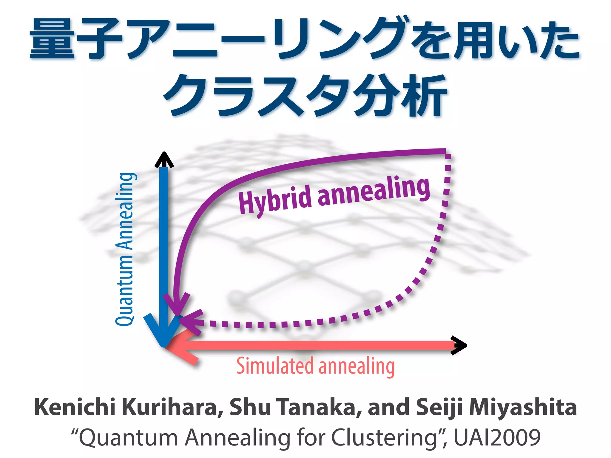
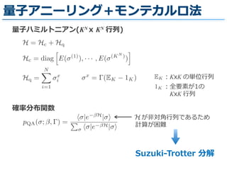
29. 数値計算結果 40 60 80 100 6.754 6.758 6.762 x 10 5 iteration minjE(σj) 40 60 80 100 6.756 6.758 6.76 6.762 6.764 6.766 6.768 x 10 5 iteration Ej[E(σj)] 40 60 80 100 0.6 0.8 1 iteration Ej[˜s(σj,σj+1)] MNIST with MoG rβ = 1.05 QA rΓ =1.02; f2 QA rΓ =1.05; f2 QA rΓ =1.10; f∗ QA rΓ =1.20; f∗ SA 40 60 80 100 1.78 1.8 1.82 1.84 1.86 x 10 5 iteration minjE(σj) 40 60 80 100 1.8 1.82 1.84 1.86 1.88 x 10 5 iteration Ej[E(σj)] 40 60 80 100 0 0.5 1 iteration Ej[˜s(σj,σj+1)] Reuters with LDA rβ = 1.05 QA rΓ =1.02; f2 QA rΓ =1.05; f2 QA rΓ =1.10; f∗ QA rΓ =1.20; f∗ SA 9.6 x 10 5 minjE(σj) 9.6 x 10 5 Ej[E(σj)] 0.5 1 j[˜s(σj,σj+1)] NIPS with LDA rβ = 1.05 QA rΓ =1.02; f2 QA rΓ =1.05; f2 QA rΓ =1.10; f∗ 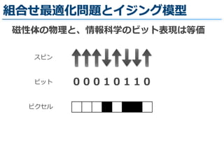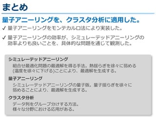MNIST(⼿手書き⽂文字認識識5000字を30個のクラスに分類) 全レイヤー中エネルギー最⼩小全レイヤーエネルギー平均レイヤー間類似度度(相関関数) スケジュール f* の場合に、 SAよりも良良い解が得られた CPU time(QA): 21.7hours CPU time(SA): 22.0hours 良良い解

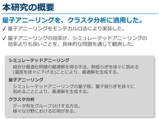
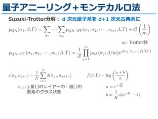
30. 数値計算結果 40 60 80 100 6.754 6.758 6.762 x 10 5 iteration minjE(σj) 40 60 80 100 6.756 6.758 6.76 6.762 6.764 6.766 6.768 x 10 5 iteration Ej[E(σj)] 40 60 80 100 0.6 0.8 1 iteration Ej[˜s(σj,σj+1)] MNIST with MoG rβ = 1.05 QA rΓ =1.02; f2 QA rΓ =1.05; f2 QA rΓ =1.10; f∗ QA rΓ =1.20; f∗ SA 40 60 80 100 1.78 1.8 1.82 1.84 1.86 x 10 5 iteration minjE(σj) 40 60 80 100 1.8 1.82 1.84 1.86 1.88 x 10 5 iteration Ej[E(σj)] 40 60 80 100 0 0.5 1 iteration Ej[˜s(σj,σj+1)] Reuters with LDA rβ = 1.05 QA rΓ =1.02; f2 QA rΓ =1.05; f2 QA rΓ =1.10; f∗ QA rΓ =1.20; f∗ SA 40 60 80 100 9.4 9.6 x 10 5 iteration minjE(σj) 40 60 80 100 9.4 9.6 x 10 5 iteration Ej[E(σj)] 40 60 80 100 0 0.5 1 iteration Ej[˜s(σj,σj+1)] NIPS with LDA rβ = 1.05 QA rΓ =1.02; f2 QA rΓ =1.05; f2 QA rΓ =1.10; f∗ QA rΓ =1.20; f∗ SA 9.4 9.45 9.5 x 10 5 minjE(σj) 9.4 9.5 9.6 x 10 5 Ej[E(σj)] 0.4 0.6 0.8 j[˜s(σj,σj+1)] NIPS with LDA rβ = 1.02 QA rΓ =1.02; f2 QA rΓ =1.05; f∗ QA rΓ =1.10; f∗ 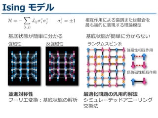REUTERSの1000記事を20トピックに分割全レイヤー中エネルギー最⼩小全レイヤーエネルギー平均レイヤー間類似度度(相関関数) スケジュール f* の場合に、 SAよりも良良い解が得られた CPU time(QA): 9.9hours CPU time(SA): 10.0hours 良良い解

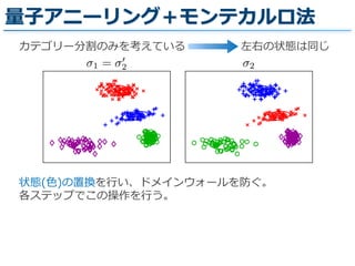
31. 数値計算結果 40 60 80 100 iteration 40 60 80 100 iteration 40 60 80 100 iteration SA 40 60 80 100 1.78 1.8 1.82 1.84 1.86 x 10 5 iteration minjE(σj) 40 60 80 100 1.8 1.82 1.84 1.86 1.88 x 10 5 iteration Ej[E(σj)] 40 60 80 100 0 0.5 1 iteration Ej[˜s(σj,σj+1)] Reuters with LDA rβ = 1.05 QA rΓ =1.02; f2 QA rΓ =1.05; f2 QA rΓ =1.10; f∗ QA rΓ =1.20; f∗ SA 40 60 80 100 9.4 9.6 x 10 5 iteration minjE(σj) 40 60 80 100 9.4 9.6 x 10 5 iteration Ej[E(σj)] 40 60 80 100 0 0.5 1 iteration Ej[˜s(σj,σj+1)] NIPS with LDA rβ = 1.05 QA rΓ =1.02; f2 QA rΓ =1.05; f2 QA rΓ =1.10; f∗ QA rΓ =1.20; f∗ SA 90 120 150 180 9.35 9.4 9.45 9.5 x 10 5 iteration minjE(σj) 90 120 150 180 9.4 9.5 9.6 x 10 5 iteration Ej[E(σj)] 90 120 150 180 0.2 0.4 0.6 0.8 iteration Ej[˜s(σj,σj+1)] NIPS with LDA rβ = 1.02 QA rΓ =1.02; f2 QA rΓ =1.05; f∗ QA rΓ =1.10; f∗ QA rΓ =1.20; f∗ SA 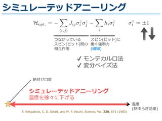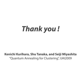e 6: Comparison between SA and QA varying annealing schedule. rΓ, f2 and f∗ in legends corres The left-most column shows what SA and QA found. QA with f∗ always found better results th NIPSの1684記事を20トピックに分割全レイヤー中エネルギー最⼩小全レイヤーエネルギー平均レイヤー間類似度度(相関関数) スケジュール f* の場合に、 SAよりも良良い解が得られた CPU time(QA): 62.5hours CPU time(SA): 62.8hours 良良い解

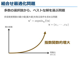
32. 数値計算結果 40 60 80 100 iteration 40 60 80 100 iteration 40 60 80 100 iteration SA 40 60 80 100 9.4 9.6 x 10 5 iteration minjE(σj) 40 60 80 100 9.4 9.6 x 10 5 iteration Ej[E(σj)] 40 60 80 100 0 0.5 1 iteration Ej[˜s(σj,σj+1)] NIPS with LDA rβ = 1.05 QA rΓ =1.02; f2 QA rΓ =1.05; f2 QA rΓ =1.10; f∗ QA rΓ =1.20; f∗ SA 90 120 150 180 9.35 9.4 9.45 9.5 x 10 5 iteration minjE(σj) 90 120 150 180 9.4 9.5 9.6 x 10 5 iteration Ej[E(σj)] 90 120 150 180 0.2 0.4 0.6 0.8 iteration Ej[˜s(σj,σj+1)] NIPS with LDA rβ = 1.02 QA rΓ =1.02; f2 QA rΓ =1.05; f∗ QA rΓ =1.10; f∗ QA rΓ =1.20; f∗ SA 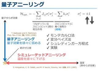e 6: Comparison between SA and QA varying annealing schedule. rΓ, f2 and f∗ in legends corres The left-most column shows what SA and QA found. QA with f∗ always found better results th how QA’s performance for each problem like this . However, it is worth trying to develop QA- algorithms for different models, e.g. Bayesian rks, by different quantum effect Hq. The pro- algorithm looks like genetic algorithms in terms ning multiple instances. Studying their relation- s also interesting future work. Tadashi Kadowaki and Hidetoshi Nishimori. Qua nealing in the transverse Ising model. Physica E, 58:5355 – 5363, 1998. S. Kirkpatrick, C. D. Gelatt, and M. P. Vecchi. O tion by simulated annealing. Science, 220(45 680, 1983. Percy Liang, Michael I. Jordan, and Ben Tas permutation-augmented sampler for DP mixtu NIPSの1684記事を20トピックに分割全レイヤー中エネルギー最⼩小全レイヤーエネルギー平均レイヤー間類似度度(相関関数) スケジュール f* の場合に、 SAよりも良良い解が得られた CPU time(QA): 62.5hours CPU time(SA): 62.8hours 良良い解

33. 量量⼦子・熱同時アニーリング温度度(熱ゆらぎ)Simulated Annealing QuantumAnnealing 量量⼦子ゆらぎ最適解を得る経路路：f* 温度度を速く下げて、その後量量⼦子項を速く弱める効率率率が悪い経路路：f2

34. まとめ量量⼦子アニーリングを、クラスタ分析に適⽤用した。 ✔ 量量⼦子アニーリングをモンテカルロ法により実装した。 ✔ 量量⼦子アニーリングの効率率率が、シミュレーテッドアニーリングの　効率率率よりも良良いことを、具体的な問題を通じて観測した。シミュレーテッドアニーリング　組合せ最適化問題の最適解を得る⼿手法。熱揺らぎを徐々に弱める　(温度度を徐々に下げる)ことにより、最適解を⽣生成する。量量⼦子アニーリング　シミュレーテッドアニーリングの量量⼦子版。量量⼦子揺らぎを徐々に　弱めることにより、最適解を⽣生成する。クラスタ分析　データ列列をグループ分けする⽅方法。　様々な分野における応⽤用がある。

35. Thank you ! Kenichi Kurihara, Shu Tanaka, and Seiji Miyashita “Quantum Annealing for Clustering”, UAI2009

量子アニーリングを用いたクラスタ分析

You are reading a preview.

量子アニーリングを用いたクラスタ分析

More Related Content

Viewers also liked

More from Shu Tanaka

Featured

Related Books

Related Audiobooks