The document discusses projectile and circular motion. It provides equations to describe the trajectory, velocity, and forces involved in curved motion. For projectile motion, the initial position and velocity along with gravity determine the trajectory. Circular motion requires a centripetal force directed toward the center, which depends on the object's mass, velocity, and distance from the center. Examples are included to calculate parameters for the moon orbiting earth and an object in circular motion like a fairground ride.

1. Curved motion

2. Overview
The trajectory and velocity of an object is fully determined by…
1. Its initial place 푠 0
2. Its initial velocity 푣 0
3. The present overall force field Σ퐹
Curved motion 2
푣 0
Σ퐹
푠 0
푣 0
푣 0
푠 0 Σ퐹
푣 0
푠 0
Σ퐹
Uniform Σ퐹 ON the
same working line as 푣 0
= Linear motion
Uniform Σ퐹 NOT ON the
same working line as 푣 0
= Projectile motion
Σ퐹 always directed to ONE
single point + constant 푣 .
= Circular motion

3. Velocity change Δ푣 as a vector
Curved motion 3
푣 0
Σ퐹
푣 0
푣 0
Σ퐹
푣 0
Σ퐹
Δ푣 = 푎 Δ푡 =
1
푚
Σ퐹 Δ푡 The velocity always changes in the direction of the overall force
Δ푣
푣 1
Δ푣
푣 1
푣 1
푣 2
Δ푣
Δ푣
Δ푣
푣 1
Verify in the pictures that always Δ푣 ∕∕ Σ퐹
Difficult because Σ퐹
changes direction
during Δ푡
So Δ푡 must be small

4. Projectile (ballistic) motion
Curved motion 4
푣 0
ℎ1 ℎ0
푣 1
푣 2
퐹 푊
Range
Trajectory
Assumption: Σ퐹 = 퐹 푊 (only uniform downwards weight, no air resistance)

5. Projectile motion, scalar treatment - I
2 + 푚푔ℎ1 ⇒
2 + 푔ℎ0 =
2 + 푔ℎ1
Curved motion 5
푣 0
ℎ1 ℎ0
푣 1
푣 2
퐹 푊
Use the energy conservation law 퐸0 = 퐸1 = 퐸2
Range
Trajectory
퐸푝0 + 퐸푘0 = 퐸푝1 + 퐸푘1 ⇒
1
2
2 + 푚푔ℎ0 =
푚푣0
1
2
푚푣1
1
2
푣0
1
2
푣1
To calculate the maximum height, apply 퐸0 = 퐸1
4 unknowns, so 3 must be known

6. Projectile motion, scalar treatment - II
2 + 푚푔 ∙ 0 ⇒
2 + 푔ℎ0 =
2
Curved motion 6
푣 0
푣 1
ℎ1 ℎ0
푣 2
퐹 푊
Range
Trajectory
퐸푝0 + 퐸푘0 = 퐸푝2 + 퐸푘2 ⇒
1
2
2 + 푚푔ℎ0 =
푚푣0
1
2
푚푣2
1
2
푣0
1
2
푣2
To calculate the final velocity, apply 퐸0 = 퐸2
3 unknowns, so 2 must be known

7. Projectile motion, scalar treatment - III
Range
2 ⇒ 푣2 = 24.4푚푠2
Curved motion 7
푣 0
푣 1
ℎ1 ℎ0
푣 2
퐹 푊
Example: ℎ0 = 10.0푚, 푣0 = 20.0푚푠−1, 푣1 = 18.0푚푠−1
Trajectory
Maximum height:
1
2
2 + 푔ℎ0 =
푣0
1
2
2 + 푔ℎ1 ⇒
푣1
1
2
20.02 + 9.81 ∙ 10.0 =
1
2
18.02 + 9.81 ∙ ℎ1 ⇒ ℎ1 = 13.9푚
Final velocity:
1
2
2 + 푔ℎ0 =
푣0
1
2
2 + 푔ℎ2 ⇒
푣2
1
2
20.02 + 9.81 ∙ 10.0 =
1
2
푣2
Important: Scalar treatment does not solve: time values & angle values & range !

8. Projectile motion, vector treatment - I
Curved motion 8
푠푦 푣푥
퐹 푊
푣
푠
푠푥
푣푦
start
origin
Resolve 푠 , 푣 , 푎 , and 퐹 in separate 푥 & 푦 direction.
1. Make sure 푥-axis is horizontal, 푦-axis is vertical
2. Choose origin below the start point on ℎ = 0
3. Choose ‘+ directions’: to right and upwards
In that case the equations of motion can be written
independently for both directions:
푠푥 = 푠푥0 + 푣푥0 ∙ 푡 + 1
2 푎푥 ∙ 푡2
푣푥 = 푣푥0 + 푎푥 ∙ 푡
푠푦 = 푠푦0 + 푣푦0 ∙ 푡 + 1
2 푎푦 ∙ 푡2
푣푦 = 푣푦0 + 푎푦 ∙ 푡
With the correct initial values this becomes easier…
휃

9. Projectile motion, vector treatment - II
Curved motion 9
푠푦 푣푥
퐹 푊
푣
푠
푠푥
푣푦
start
origin
Choose:
푠푥0 = 0 & 푠푦0 = ℎ0
푣푥0 = 푣0퐶표푠휃 & 푣푦0 = 푣0푆푖푛휃
푎푥 = 0 & 푎푦 = −푔
Now the equations reduce to:
푠푥 = 푣푥0 ∙ 푡
푠푦 = ℎ0 + 푣푦0 ∙ 푡 − 1
2 푔 ∙ 푡2
푣푦 = 푣푦0 − 푔 ∙ 푡
And for a horizontal projection (휃 = 0)
푠푥 = 푣0 ∙ 푡
푠푦 = ℎ0 − 1
2 푔 ∙ 푡2
푣푦 = −푔 ∙ 푡
휃

10. Projectile motion, vector treatment - III
Curved motion 10
푣 = 20.0푚푠−1
퐹 푊
origin
Example
ℎ0 = 10.0푚, 휃 = 0.0°, 푣0 = 20.0푚푠−1
푠푥 = 20.0 ∙ 푡
푠푦 = 10 − 4.905 ∙ 푡2
푣푦 = −9.81 ∙ 푡
Time at the ground: set 푠푦 = 0 ⇒ 10 − 4.905 ∙ 푡2 = 0 ⇒ 푡 = 1.43푠
Range: 푠푥 1.43 = 20 ∙ 1.43 = 28.6푚
Final velocity: 푣푥 1.43 = 20푚푠−1 푣푦 1.43 = −9.81 ∙ 1.43 = −14.0푚푠−1
Magnitude: 푣 1.43 = 202 + 142 = 24.4푚푠−1
Angle: 휃 1.43 = 푡푎푛−1 푣푦 푣푥 = 푡푎푛−1 −14.0 20.0 = −35.0°
ℎ0

11. Projectile motion, vector treatment - IV
Curved motion 11
퐹 푊
푣 = 20.0푚푠−1
푣푥
푣푦
origin
Example
ℎ0 = 10.0푚, 휃 = 30.0°, 푣0 = 20.0푚푠−1
푣0푥 = 20퐶표푠 30° = 17.32푚푠−1
푣0푦 = 20푆푖푛 30° = 10.0푚푠−1
푠푥 = 17.32 ∙ 푡
푠푦 = 10 + 10 ∙ 푡 − 4.905 ∙ 푡2
푣푦 = 10 − 9.81 ∙ 푡
Time at highest point: set 푣푦 = 0 ⇒ 10 − 9.81 ∙ 푡 ⇒ 푡 = 1.02푠
Height of highest point: 푠푦 1.02 = 10 + 10 ∙ 1.02 − 4.905 ∙ 1.022 = 15.1푚
Time at the ground: set 푠푦 = 0 ⇒ 10 + 10 ∙ 푡 − 4.905 ∙ 푡2 = 0
4.905푡2 − 10푡 − 10 = 0 ⇒ 푡 =
10 ± 102 − 4 ∙ 10 ∙ −4.905
2 ∙ 4.905
= 2.77푠
Range: 푠푥 2.77 = 17.32 ∙ 2.77 = 48.0푚
Final velocity: 푣푥 2.77 = 17.32푚푠−1 푣푦 2.77 = 10 − 9.81 ∙ 2.77 = −17.2푚푠−1
Magnitude: 푣 2.77 = 17.322 + 17.22 = 24.4푚푠−1
Angle: 휃 2.77 = 푡푎푛−1 푣푦 푣푥 = 푡푎푛−1 −17.2 17.32 = −44.8°
ℎ0
30°

12. Projectile motion, vector treatment - V
RESULTS of the calculation
Curved motion 12
푣 = 20.0푚푠−1
퐹 푊
30.0°
ℎ0 = 10.0푚
푣 = 24.4푚푠−1
ℎ1 = 15.1푚
휃 = −35.0° 휃 = −44.8°
28.6푚
48.0푚

13. Acceleration in circular motion
푣 0
Δ휙 A
푣 1
푣 1
Δ휙
푟
Δ푠
푟
푣 0
Δ푣
B
Curved motion 13
In a circle segment: 푎푟푐 퐴퐵 = 푟 ∙ Δ휙 (푟푎푑)
If 휙 small: Δ푠 = 푟 ∙ Δ휙 ⇒ Δ휙 = Δ푠 푟
The 2 triangles are similar, so:
Δ휙(푠푚푎푙푙) =
Δ푣
푣
=
Δ푠
푟
Divide by Δ푡:
Δ푣
=
푣 ∙ Δ푡
Δ푠
푟 ∙ Δ푡
⇒ 푟
Δ푣
Δ푡
= 푣
Δ푠
Δ푡
⇒ 푟 ∙ 푎 = 푣2
푎 =
푣2
푟
Centripetal acceleration

14. Force in circular motion
푣 0
푣 1
A
B
Curved motion 14
According to Newton’s 2nd law an acceleration 푎
requires an overall force Σ퐹 = 푚푎
In other words:
An object that orbits around a point at a distance 푟
With a velocity 푣 requires an overall force:
퐹푐푝푡 = 푚푎푐푝푡 =
푚푣2
푟
Centripetal force
퐹 푐푝푡

15. Force in circular motion – Example I
Curved motion 15
Moon circles around Earth
Distance Earth - Moon 푟 = 384.4 ∙ 106푚
Period 푇 = 27.32푑
Mass 푚 = 7.35 ∙ 1022푘푔
푣 =
2휋푟
푇
=
2휋 ∙ 384.4 ∙ 106
27.32 ∙ 24 ∙ 3600
= 1023푚푠−1
푎푐푝푡 =
푣2
푟
=
10232
384.4 ∙ 106 = 2.724 ∙ 10−3푚푠−2
퐹푐푝푡 = 푚푎푐푝푡 = 2.002 ∙ 1020푁
This force is provided by the gravitational pull of the Earth

16. Force in circular motion – Example IIa
퐹 푁
퐹 푐푝푡 = Σ퐹
Curved motion 16
Fairground looping – lowest point
Radius 푟 = 14푚
Velocity 푣 = 24푚푠−1
Mass (you) 푚 = 65푘푔
푎푐푝푡 =
푣2
푟
=
242
14
= 41푚푠−2 퐹푐푝푡 = 푚푎푐푝푡 = 2.67 ∙ 103푁
Weight 퐹푊 = 0.64 ∙ 103푁 works in the wrong direction!
A normal force 퐹푁 = 2.67 ∙ 103 + 0.64 ∙ 103 = 3.3 ∙ 103푁
is required to provide the necessary 퐹푐푝푡
“you feel the chair pressing you upwards”
퐹 푊

17. Force in circular motion – Example IIb
You are 2 × 14푚 higher now and your velocity equals 5.2푚푠−2
in stead of 24푚푠−1 . Energy conservation law, check it yourself!
퐹 푁
퐹 푐푝푡 = Σ퐹
Curved motion 17
Fairground looping – highest point
Radius 푟 = 14푚
Velocity 푣 = 5.2푚푠−1
Mass (you) 푚 = 65푘푔
푎푐푝푡 =
푣2
푟
=
5.22
14
= 1.9푚푠−2 퐹푐푝푡 = 푚푎푐푝푡 = 126푁
Weight 퐹푊 = 638푁 works in the correct direction, but is too much!
An upwards normal force 퐹푁 = 638 − 126 = 5.1 ∙ 102푁
is required to compensate weight and provide the necessary 퐹푐푝푡
“you are saved by the braces (belts)”
퐹 푊

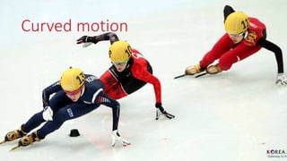
18. Force in circular motion – Example III
퐹 푖푐푒
Curved motion 18
Short track skating
Radius 푟 = 8.0푚
Velocity 푣 = 10푚푠−1
Mass 푚 = 65푘푔
푎푐푝푡 =
푣2
푟
=
102
8.0
= 12.5푚푠−2
퐹푐푝푡 = 푚푎푐푝푡 = 813푁
Weight 퐹푊 = 638푁 works downwards!
Construct a free body diagram to find the contact force
by the ice on the skates.
With 1cm ≜ 200푁 this yields 퐹푖푐푒 = 1.0 ∙ 103푁
Or calculate it algebraically with Pythagoras.
푡푎푛 휃 =
퐹푊
퐹푐푝푡
=
푚푔
푚푣2 푟
=
푔푟
푣2 = 0.785 ⇒ 휃 = 38°
Or measure it in the free body diagram
Vectors must be
퐹 on scale! 푊
퐹 푐푝푡
휃

19. Satellite orbits
In case of satellites orbiting a planet (Earth), the 퐹푐푝푡
Is provided by the gravitational force between to masses:
Curved motion 19
퐹푔 = 퐺
푀 ∙ 푚
푟2
Newton’s law of gravitation
푀
Typically large
푚
Typically small
퐹
푣
푟
Inverse
square law
Gravitational constant 퐺 = 6.67384 ∙ 10−11푚3푘푔−1푠−2

20. Kepler’s 3rd law
Curved motion 20
퐹푔 = 퐹푐푝푡 ⇒ 퐺
푀 ∙ 푚
푟2 =
푚 ∙ 푣2
푟
⇒ 퐺 ∙ 푀 = 푟 ∙ 푣2
ℎ
푅푝
푟
Substitute: 푣 =
2휋푟
푇
퐺 ∙ 푀 = 푟 ∙
2휋푟
푇
2
= 4휋2 푟3
푇2 ⇒
푟3
푇2 =
퐺푀
4휋2 = 푐표푛푠푡푎푛푡
푇
Attention: 푟 = 푅푝 + ℎ. Always add the planet’s radius to the orbiting altitude to get the correct radius

21. Kepler’s 3rd law - Example
Earth
Mass 푀 = 5.976 ∙ 1024푘푔
Radius 푅푝 = 6.378 ∙ 106
Siderial rotation
푇 = 23.93ℎ
period
Curved motion 21
Calculate the altitude above the Earth’s surface
of geostationary satellites
푟3
푇2 =
퐺푀
4휋2 =
6.67384 ∙ 10−11 ∙ 5.976 ∙ 1024푘푔
4휋2 = 1.010 ∙ 1013푚3푠−2
푟3 = 1010 ∙ 1013 ∙ 23.93 ∙ 3600 2 = 7.4975 ∙ 1022
푟 =
3
2.355 ∙ 1023 = 42.167 ∙ 106푚
ℎ = 푟 − 푅푝 = 42.167 ∙ 106 − 6.378 ∙ 106 = 35.79 ∙ 106 푚
wikimedia

22. END
Disclaimer
This document is meant to be apprehended through professional teacher mediation (‘live in class’)
together with a physics text book, preferably on IB level.
Curved motion 22