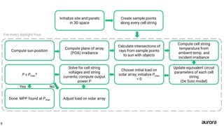
Cell String-Level Energy Production Simulation with Aurora is powerful software used to create over 10k solar projects per week. It provides the most granular submodule-level modeling to capture partial shading, bypass diodes, and cell string-level power electronics in PV systems. The simulation initializes site and panel configurations in 3D space, computes irradiance and temperature for each cell string, and models each string as an electrical circuit to solve for maximum power point at each hour. Results show cell string-level simulation can improve energy production and lifetime energy bill savings accuracy by 1-4% compared to module-level simulation due to its ability to account for unique string configurations, bypass diodes, and cell string optimizers.

1. Cell String-Level Energy Production
Simulation with Aurora

2. Powerful software for residential and commercial solar sales and design
Founded 2013
Used to create over 10k projects per week
2

3. Aurora’s Feature Set
• 3D modeling with LIDAR and Streetview measurements
• Automatic obstruction detection with computer vision
• Bankable shade reports using integrated shading engine
• Residential and commercial financial analysis
• Automatic optimal PV system designer
• NEC design validation report
• Breakdown of system losses
• Sales proposal tool
• Electrical line drawings
• Submodule performance simulation engine → today’s focus
3

4. Simulation
Types
• Array-level
• Module-level
• Submodule-level
4

5. A Look Inside a Solar Panel
5

6. Bypass Diodes and Partial Shading
6
No bypass diodes
Shade knocks out
entire string of modules
One bypass diode
Shade knocks out single module
Three bypass diodes
Shade knocks out single cell string

7. Submodule-Level Modeling
• Most granular model to capture partial shading, bypass diodes, and cell string-level
power electronics in modern PV systems
– Compute irradiance (S) on and temperature (T) of every cell string in the array
– Model each cell string as a circuit, adjust params given (S,T) at a given hour
– Solve for MPP by solving (larger) nonlinear circuit
7

8. Initialize site and panels
in 3D space
Compute sun position
Calculate intersections of
rays from sample points
to sun with objects
Create sample points
along every cell string
Compute plane of array
(POA) irradiance
Compute cell string
temperature from
ambient temp. and
incident irradiance
For every daylight hour
Update equivalent circuit
parameters of each cell
string
(De Soto model)
Solve for cell string
voltages and string
currents; compute output
power P
Choose initial load on
solar array; initialize Pmax
= 0
P ≤ Pmax?
Done: MPP found at Pmax Adjust load on solar array
Yes No
8

9. 9

10. Energy Production Results
10
Design
Annual Production,
Module-Level [MWh]
Annual Production,
Submodule-Level [MWh]
% Difference
3 ft spacing, 154.3 kW 189.50 191.76 1.19%
2.5 ft spacing, 158.9 kW 193.29 196.11 1.45%
2 ft spacing, 177.7 kW 212.66 217.41 2.21%
1.5 ft spacing, 201.0 kW 232.67 241.19 3.60%
Module-Level,
1.5 ft spacing
Submodule-
Level, 1.5 ft
spacing

11. Financial Analysis Results
11
Design
Lifetime Energy Bill Savings,
Module-Level [$]
Lifetime Energy Bill Savings,
Submodule-Level [$]
% Difference
3 ft spacing, 154.3 kW 575,484 584,718 1.59%
2.5 ft spacing, 158.9 kW 584,958 596,464 1.95%
2 ft spacing, 177.7 kW 640,086 659,581 3.00%
1.5 ft spacing, 201.0 kW 691,797 726,511 4.90%

12. Why Else Does Submodule Simulation
Matter?
12

13. Unique Cell String Configurations
vs.
13
Module power
90 W + 90 W - 5 W = 175 W
Module power
90 W + 90 W + 45 W - 5 W = 220 W

14. Cell String-Level Optimizers
vs.
14
Module power
90 W + 90 W - 5 W = 175 W
Module power
90 W + 90 W + 45 W = 225 W

15. Cell String Optimization
15
Without cell string-level optimizers
6.45 MWh
With cell string-level optimizers
7.17 MWh

16. Accuracy
16
NREL Site
Average
Annual %
Error
Andre Agassi Prep Academy 2.16%
Sanyo Mono Test Array 1.26%
RSF1 2.35%
RSF2 0.2%
Science and Technology Facility 1.8%
Month
Percent
Error [%]
Jan 1.9
Feb 0.6
Mar 1.3
Apr -0.1
May -1.0
Jun -0.1
Jul -0.4
Aug -0.4
Sep -0.7
Oct 0.0
Nov 0.4
Dec 3.4

17. Takeaways
• Cell string-level simulation
important for assessing
performance implications of:
– Bypass diodes
– Unique cell string
configurations
– Cell string-level optimizers
• 1-3% improvement in
accuracy can have significant
impact on financial results
17

18. Additional Resources
blog.aurorasolar.com
18
/aurorasolarinc /company/aurora-solar
@aurorasolarinc/AuroraSolarInc
help.aurorasolar.com
www.aurorasolar.com

19. Backup
19