SlideShare a Scribd company logo
1 of 16
Download to read offline
Advanced Finite Element Analysis Ravishankar Venkatasubramanian
Page 1
Project Report: Advanced Finite Element Analysis
Introduction:
In this project, we explore problems pertinent to two major systems:
1. Dynamics Analysis
2. Non Linear Analysis
Dynamic analysis are real-world problems which are analyzed by understanding either the mode shapes
and Eigen values and then using this data to find out a specific response, or by the method of time
integration, which is a more direct method of solving these problems. Although time integration is a
direct method, the mathematics involved in its use is tedious that it cannot be used for large number of
degrees of freedom (DOFs). Hence, we use modal superposition to calculate the response for large
number of DOFs. In this project, we will discuss the application of modal superposition on a cantilever
plate.
Non-Linear analysis is subdivided into two major categories:
1. Geometric Non-Linearity.
2. Material Non-Linearity
In Geometric Non-Linearity, the non-linearity exists in the way the deformation occurs. Large
deformation for example is one of the examples for Geometric Non-linearity. In this project, we discuss
and analyze one example of geometric non-linearity. On the other hand, in Material Non-Linearity, the
non-linearity exists in the properties of the material, that is, the material could be Hyperelastic, or could
be Elastoplastic. We will discuss one example on Material Non-Linearity as well.
Let us begin our discussion with an example in Dynamics Analysis:
Example 1: Dynamics Analysis (Normal Modes and Frequency Response Analysis)
References:
1. http://www.scc.kit.edu/scc/sw/msc/Nas102/prob01.pdf
2. http://web.mscsoftware.com/support/online_ex/previous_nastran/nas102/prob06.pdf
For a flat plate as shown below, perform Modal Analysis to determine the first five modes of vibration,
and its corresponding mode shapes.
Figure 1: Description of Length and Breadth Dimensions and mesh system in NASTRAN Analysis
Advanced Finite Element Analysis Ravishankar Venkatasubramanian
Page 2
Figure 2: Material Properties
The system is excited by a 0.1 psi pressure load over the total surface of the plate and a 1.0 lb. force at
a corner of the tip lagging 45°. Use a modal damping of ξ = 0.03. Use a frequency step of 20 Hz between
a range of 20Hz and 1000 Hz. Perform Modal Frequency Response analysis for the mentioned loads
and boundary conditions:
Figure 3: Boundary Conditions and Load
Solution:
We use ANSYS Workbench 17.0 for the analysis and simulation. The solution was first attempted using
3D- Hexahedral elements. The initial analysis to be done was Modal Analysis. A fixed support boundary
condition is applied to the system, as shown in Figure 4.
Advanced Finite Element Analysis Ravishankar Venkatasubramanian
Page 3
Figure 4: Boundary Condition for Eigen Value Analysis
After the boundary conditions are applied, the number of modes to be found are written in the Analysis
settings tab, as shown in Figure 5:
Figure 5: Analysis Settings – Modal Analysis
After this step, Eigen value analysis is run to find out the Mode shapes (Eigen vectors) and Eigen Values
(Natural Frequency), as shown in Figure 6 and Figure 7.
Figure 6: Natural Frequency for each mode
Advanced Finite Element Analysis Ravishankar Venkatasubramanian
Page 4
Figure 7: Mode Shape 1 for a Natural Frequency of 131.79 Hz.
These answers of fundamental frequencies from Figure 6 match closely with the answers obtained in
the NASTRAN Example problem (from reference), as shown in Figure 8 (Natural Frequency circled in
blue):
Figure 8: Eigen Values and Natural Frequencies from NASTRAN Example Problem.
Varying the mesh density and the type of element (From Hexahedral to Tetrahedral) gives tiny change
in Modal Frequency, which is not highly significant.
Using these Eigen Values, we now move on to Frequency Response Analysis. In frequency response
analysis, we use the Eigen values to find out Frequency response as a function of these mode shapes
and modal frequencies. This method saves a lot of time compared to the direct method. Figure 9
provides the geometry, and the requisite boundary conditions applied.
Advanced Finite Element Analysis Ravishankar Venkatasubramanian
Page 5
Figure 9: Boundary Conditions on the Model
Initially, hexahedral elements are used for the analysis, and the mesh density is at its coarsest. This
analysis is run with the mentioned damping ratio and the frequency range, with mentioned steps in
frequency is taken, as shown in Figure 10.
Figure 10: Analysis Settings
Advanced Finite Element Analysis Ravishankar Venkatasubramanian
Page 6
With the mentioned Analysis settings, the Frequency Response Analysis (FRA) was run. The FRA
peaks are shown in Figure 11:
Figure 11: FRA peaks for Hexahedral Elements
The FRA peaks show that the displacement amplitude is highest near the resonance frequencies between
10Hz- 1000Hz. This is expected for the question as instability generally exists near the resonant
frequencies. The value of displacement can be further refined by using a finer mesh. Testing has also
been done using Tetrahedral mesh, and the displacement has been found to be close to the answer
mentioned in the NASTRAN Manual (Figure 12) for fine Hexahedral mesh. Hexahedral elements have
more nodes, and hence can handle bending better than Tetrahedral elements. A finer mesh provides
closer interpolation values, and more accurate results.
Figure 12: PATRAN Results from Reference for FRA
Advanced Finite Element Analysis Ravishankar Venkatasubramanian
Page 7
FRA analysis for higher number of solution intervals, i.e., higher number of frequencies between 20Hz-
1000Hz provides a smoother curve with higher accuracy of results. But these results cannot be
compared with the results from Figure 12, which is based on a solution interval of 49.
For Tetrahedral elements, the FRA provides a higher displacement, since the tetrahedral elements
cannot handle bending and oscillatory movements as effectively as Hexahedral elements, there is a
slightly higher displacement, as shown in Figure 13.
Figure 13: FRA peaks for Tetrahedral Elements
The system is a plate system, and cannot be modeled as a 1D system, and hence, we restrict its modeling.
With increase in mesh density, there is an increase in accuracy. Hence, the most accurate mesh to use
in this case is a Fine-Hexahedral mesh.
Example 2: (Large Deformation; Geometric Non-Linearity)
Reference: http://support.midasnfx.com/files/NAFEMS-PDF/Z-shaped%20cantilever.pdf
Figure 14 shows a Z-shaped cantilever laid along the oblique line of 45˚. The total load P at all the
points on the free end D in the positive Z-direction is conservative (non-follower load). The material
properties are also given.
Figure 14: Z- Shaped Cantilever
Advanced Finite Element Analysis Ravishankar Venkatasubramanian
Page 8
Solution:
This system is designed on ANSYS Workbench 17.0 using the Design Modeler. The model was initially
modeled as a 3D system, and later modeled as a 2D system and a 1D system. We will discuss about the
results of each system in detail.
Figure 15: Hexahedral Coarse Mesh
Figure 16 shows details of the boundary conditions. The fixed support boundary condition and Force is
applied in a ramped fashion, over a period of time.
Figure 16: Boundary Conditions on the Z-Shaped Cantilever
Advanced Finite Element Analysis Ravishankar Venkatasubramanian
Page 9
Figure 17: Application of Ramped Force
Ramped force is essential to make sure that the system does not collapse due to sudden application of
forces up to 4000N.
Figure 18: Analysis Settings
The number of steps is set to 100 to obtain an accurate non-linear solution. The other controls are set to
program controlled as the question does not mention any other specific changes to make to the system.
The final deformation, at Load = 4000N is shown in Figure 19:
Advanced Finite Element Analysis Ravishankar Venkatasubramanian
Page 10
Figure 19: Directional Deformation of the system at 4000N Load
A graph is drawn with displacement in the X-Axis and Load in the Y-axis, to get an idea about how the
system deforms with increasing force. The displacement rapidly increases with load for the first 500N.
After this force, the deformation has reached around 100mm, where the mid-section of the Z-shaped
cantilever causes ‘tension stiffening’, as shown in Figure 20. This tension stiffening continues all the
way upto the load of 4000N, and it can be see that there is very less displacement (43mm) over a large
amount of force (3500N). This can be attributed solely to the stiffening in the mid-section of the Z
shaped cantilever. Please note that the deformation shown in Figure 19 is only for the tip of the
cantilever.
Figure 20: Tip Displacement vs Load (Z Shaped Cantilever)
This graph is compared with the graph obtained from the Midas-NFX reference, shown in Figure 20.
0
500
1000
1500
2000
2500
3000
3500
4000
4500
0 20 40 60 80 100 120 140 160
Load(N)
Tip Displacement (mm)
Tip Displacement vs Load
Advanced Finite Element Analysis Ravishankar Venkatasubramanian
Page 11
Figure 21: Tip Displacement vs Displacement (Midas-NFX)
Comparing both Figure 20 and Figure 21, we can conclude that the graphs are almost the same.
Increasing the mesh density in both 3D and 1D has not provided a significant increase in the accuracy
of the system. This is probably because the system is well equipped to handle bending as such, and the
slow increase in displacement due to tension stiffening has provided sufficient iterations to weed out
any numerical errors, which might creep in the analysis. The 3D Hexahedral elements can handle
bending effectively, and hence, provide accurate results. Figure 22, 23 show pictures of the final
deformation in both 2D and 1D systems.
Figure 22: Tip Deformation – Quadrilateral Shell Elements
Advanced Finite Element Analysis Ravishankar Venkatasubramanian
Page 12
Figure 23: Tip Deformation – 1D Beam Elements
As seen from Figure 22, 1D beam elements can handle bending effectively, and hence, the deformation
at the tip matches with 3D Tetrahedral/Hexahedral elements. 2D triangular and Quadrilateral elements
on the other hand, cannot handle bending as effectively as beam elements, and provide slightly more
deformation. This is seen in Figure 21. There is no significant change in tip displacement with mesh
density, and hence, that has not been discussed in detail. For further information, the attached input files
provide 3 different mesh densities, along with all element types (3D, 2D and 1D).
The solution has been compared with the reference Midas-NFX, and has been found to match with the
prescribed result.
Example 3: (Material Non-Linearity: Elasto-Plastic Material)
Reference: http://www.scc.kit.edu/scc/sw/msc/Nas103/Workshop_6.pdf
Figure 24: Diagram of Problem
L=50, W=10, T=0.1.
The material used in this system has the following properties:
Young’s Modulus = 3.0E+6, Poisson’s Ratio = 0.25, Tangent Modulus = 30303, Yield Stress = 850.
Advanced Finite Element Analysis Ravishankar Venkatasubramanian
Page 13
Find the Elastic and Plastic Strain at the end of the loading. The loading cycle is:
1. Load P=800
2. Load P= 1000
3. Unload P= 950
4. Unload P=0
Solution:
The modeling can be done by using a quarter of the model (symmetry), and it will yield the same result
with a lesser time duration involved. But for this problem, we use a system which has the entire bar.
Figure 25 shows the meshed bar, with a coarse hexahedral mesh.
Figure 25: Meshed Part – Hexahedral Mesh
We expect, from the loading pattern that the material yields between 1 and 2 seconds, since the Yield
stress is 850. After yielding, the material will maintain its plastic nature, even if it unloads, as done in
t=3 and t=4. The loading history is shown in Figure 26 (This is because the stress is
F/A=Load/(10*0.1)=> Stress = Load).
Figure 26: Load curve with time
Advanced Finite Element Analysis Ravishankar Venkatasubramanian
Page 14
The boundary conditions applied on the system are shown in Figure 27.
Figure 27: Application of Boundary Conditions
The analysis is run, and the requested outputs are equivalent plastic strain, the total strain in the body
and the equivalent von-mises stress. The analysis is run under these conditions. Applying a fixed
boundary condition on one end provides a system which is constrained, and the simulation can proceed
as expected. The system is the same as the one where the tensile load is applied to both ends.
The equivalent plastic strain is shown in Figure 28:
Figure 28: Equivalent Plastic Strain in the system at t=4s (Final)
The system shows an equivalent plastic strain of 5.73mm, which is the same as plastic strain obtained
when the load is 1000.
Advanced Finite Element Analysis Ravishankar Venkatasubramanian
Page 15
The graph between time and equivalent plastic strain is:
Figure 29: Plastic Strain vs Time
The plastic strain remains constant in unloading, as expected, as all the elastic strain is dissipated in
unloading.
The graph between time and Equivalent total strain is:
Figure 30: Total Strain vs Time
The total strain reduces over time in the unloading process as the elastic strain is dissipated over time
during the unloading procedure. Now, we can draw a graph between the equivalent stress and plastic
strain.
Figure 31: Plastic Strain and Equivalent Stress
0
200
400
600
800
1000
1200
-0.001 0 0.001 0.002 0.003 0.004 0.005 0.006 0.007
Plastic Strain vs Equivalent Stress
Advanced Finite Element Analysis Ravishankar Venkatasubramanian
Page 16
This graph can now be compared with Figure 32, which is the graph between Plastic Strain and
Equivalent stress in the reference:
Figure 32: Plastic Strain vs Stress (Reference Material)
As seen in this system, we can say that the solution is an almost perfect match. Increasing the mesh
density provides more accuracy in the system, but changing the element type from 3D to 2D will not
cause much improvement in results. This is because Hexahedral or any element in the 3D domain can
handle stretching efficiently. Hence, this system can be meshed with any element, 3D, 2D or 1D to get
effective results.

More Related Content

What's hot

INTRODUCTION TO FINITE ELEMENT ANALYSIS
INTRODUCTION TO FINITE ELEMENT ANALYSISINTRODUCTION TO FINITE ELEMENT ANALYSIS
INTRODUCTION TO FINITE ELEMENT ANALYSIS
Achyuth Peri
 

What's hot (18)

Reliability Analysis of the Sectional Beams Due To Distribution of Shearing S...
Reliability Analysis of the Sectional Beams Due To Distribution of Shearing S...Reliability Analysis of the Sectional Beams Due To Distribution of Shearing S...
Reliability Analysis of the Sectional Beams Due To Distribution of Shearing S...
 
M1
M1M1
M1
 
Higher-Order Squeezing of a Generic Quadratically-Coupled Optomechanical System
Higher-Order Squeezing of a Generic Quadratically-Coupled Optomechanical SystemHigher-Order Squeezing of a Generic Quadratically-Coupled Optomechanical System
Higher-Order Squeezing of a Generic Quadratically-Coupled Optomechanical System
 
6 Machine design theories of failure
6 Machine design theories of failure6 Machine design theories of failure
6 Machine design theories of failure
 
Intro to fea software
Intro to fea softwareIntro to fea software
Intro to fea software
 
Dr.R.Narayanasamy - Mohr's circle and Formability
Dr.R.Narayanasamy - Mohr's circle and FormabilityDr.R.Narayanasamy - Mohr's circle and Formability
Dr.R.Narayanasamy - Mohr's circle and Formability
 
Theories of failure_scet
Theories of failure_scetTheories of failure_scet
Theories of failure_scet
 
Examining Non-Linear Transverse Vibrations of Clamped Beams Carrying N Concen...
Examining Non-Linear Transverse Vibrations of Clamped Beams Carrying N Concen...Examining Non-Linear Transverse Vibrations of Clamped Beams Carrying N Concen...
Examining Non-Linear Transverse Vibrations of Clamped Beams Carrying N Concen...
 
Lec10 finite element_beam_structures 2
Lec10 finite element_beam_structures 2Lec10 finite element_beam_structures 2
Lec10 finite element_beam_structures 2
 
E04701035045
E04701035045E04701035045
E04701035045
 
FEA_project1
FEA_project1FEA_project1
FEA_project1
 
Theories of failure
Theories of failureTheories of failure
Theories of failure
 
theory of failure
theory of failuretheory of failure
theory of failure
 
LabReport5
LabReport5LabReport5
LabReport5
 
FREQUENCY RESPONSE ANALYSIS OF 3-DOF HUMAN LOWER LIMBS
FREQUENCY RESPONSE ANALYSIS OF 3-DOF HUMAN LOWER LIMBSFREQUENCY RESPONSE ANALYSIS OF 3-DOF HUMAN LOWER LIMBS
FREQUENCY RESPONSE ANALYSIS OF 3-DOF HUMAN LOWER LIMBS
 
theories of failure
theories of failure theories of failure
theories of failure
 
Multi-Objective Genetic Topological Optimization for Design of composite wall...
Multi-Objective Genetic Topological Optimization for Design of composite wall...Multi-Objective Genetic Topological Optimization for Design of composite wall...
Multi-Objective Genetic Topological Optimization for Design of composite wall...
 
INTRODUCTION TO FINITE ELEMENT ANALYSIS
INTRODUCTION TO FINITE ELEMENT ANALYSISINTRODUCTION TO FINITE ELEMENT ANALYSIS
INTRODUCTION TO FINITE ELEMENT ANALYSIS
 

Similar to Linear Dynamics and Non-Linear Finite Element Analysis using ANSYS Workbench

1 Aminullah Assagaf_Estimation-of-domain-of-attraction-for-the-fract_2021_Non...
1 Aminullah Assagaf_Estimation-of-domain-of-attraction-for-the-fract_2021_Non...1 Aminullah Assagaf_Estimation-of-domain-of-attraction-for-the-fract_2021_Non...
1 Aminullah Assagaf_Estimation-of-domain-of-attraction-for-the-fract_2021_Non...
Aminullah Assagaf
 
2016 Fall ME 7210 Elasticity and Plasticity Final Project
2016 Fall ME 7210 Elasticity and Plasticity Final Project2016 Fall ME 7210 Elasticity and Plasticity Final Project
2016 Fall ME 7210 Elasticity and Plasticity Final Project
Joey F An
 
Nano Scale Roughness Quantification
Nano Scale Roughness QuantificationNano Scale Roughness Quantification
Nano Scale Roughness Quantification
Pratham Ghael
 
Ijarcet vol-2-issue-7-2273-2276
Ijarcet vol-2-issue-7-2273-2276Ijarcet vol-2-issue-7-2273-2276
Ijarcet vol-2-issue-7-2273-2276
Editor IJARCET
 
Ijarcet vol-2-issue-7-2273-2276
Ijarcet vol-2-issue-7-2273-2276Ijarcet vol-2-issue-7-2273-2276
Ijarcet vol-2-issue-7-2273-2276
Editor IJARCET
 

Similar to Linear Dynamics and Non-Linear Finite Element Analysis using ANSYS Workbench (20)

Steady state CFD analysis of C-D nozzle
Steady state CFD analysis of C-D nozzle Steady state CFD analysis of C-D nozzle
Steady state CFD analysis of C-D nozzle
 
FEA Report
FEA ReportFEA Report
FEA Report
 
Gx3612421246
Gx3612421246Gx3612421246
Gx3612421246
 
Transfer Functions and Linear Active Networks Using Operational Amplifiers
Transfer Functions and Linear Active Networks Using Operational AmplifiersTransfer Functions and Linear Active Networks Using Operational Amplifiers
Transfer Functions and Linear Active Networks Using Operational Amplifiers
 
How to deal with the annoying "Hot Spots" in finite element analysis
How to deal with the annoying "Hot Spots" in finite element analysisHow to deal with the annoying "Hot Spots" in finite element analysis
How to deal with the annoying "Hot Spots" in finite element analysis
 
1 Aminullah Assagaf_Estimation-of-domain-of-attraction-for-the-fract_2021_Non...
1 Aminullah Assagaf_Estimation-of-domain-of-attraction-for-the-fract_2021_Non...1 Aminullah Assagaf_Estimation-of-domain-of-attraction-for-the-fract_2021_Non...
1 Aminullah Assagaf_Estimation-of-domain-of-attraction-for-the-fract_2021_Non...
 
2016 Fall ME 7210 Elasticity and Plasticity Final Project
2016 Fall ME 7210 Elasticity and Plasticity Final Project2016 Fall ME 7210 Elasticity and Plasticity Final Project
2016 Fall ME 7210 Elasticity and Plasticity Final Project
 
Stress Analysis of Chain Links in Different Operating Conditions
Stress Analysis of Chain Links in Different Operating ConditionsStress Analysis of Chain Links in Different Operating Conditions
Stress Analysis of Chain Links in Different Operating Conditions
 
A Weighted Duality based Formulation of MIMO Systems
A Weighted Duality based Formulation of MIMO SystemsA Weighted Duality based Formulation of MIMO Systems
A Weighted Duality based Formulation of MIMO Systems
 
Comparative Study between DCT and Wavelet Transform Based Image Compression A...
Comparative Study between DCT and Wavelet Transform Based Image Compression A...Comparative Study between DCT and Wavelet Transform Based Image Compression A...
Comparative Study between DCT and Wavelet Transform Based Image Compression A...
 
I017125357
I017125357I017125357
I017125357
 
Nano Scale Roughness Quantification
Nano Scale Roughness QuantificationNano Scale Roughness Quantification
Nano Scale Roughness Quantification
 
A New Method Based on MDA to Enhance the Face Recognition Performance
A New Method Based on MDA to Enhance the Face Recognition PerformanceA New Method Based on MDA to Enhance the Face Recognition Performance
A New Method Based on MDA to Enhance the Face Recognition Performance
 
Implementation Of Geometrical Nonlinearity in FEASTSMT
Implementation Of Geometrical Nonlinearity in FEASTSMTImplementation Of Geometrical Nonlinearity in FEASTSMT
Implementation Of Geometrical Nonlinearity in FEASTSMT
 
C012621520
C012621520C012621520
C012621520
 
C012621520
C012621520C012621520
C012621520
 
Ijarcet vol-2-issue-7-2273-2276
Ijarcet vol-2-issue-7-2273-2276Ijarcet vol-2-issue-7-2273-2276
Ijarcet vol-2-issue-7-2273-2276
 
Ijarcet vol-2-issue-7-2273-2276
Ijarcet vol-2-issue-7-2273-2276Ijarcet vol-2-issue-7-2273-2276
Ijarcet vol-2-issue-7-2273-2276
 
Unit 1 notes-final
Unit 1 notes-finalUnit 1 notes-final
Unit 1 notes-final
 
MMAE 594_Report
MMAE 594_ReportMMAE 594_Report
MMAE 594_Report
 

Recently uploaded

"Lesotho Leaps Forward: A Chronicle of Transformative Developments"
"Lesotho Leaps Forward: A Chronicle of Transformative Developments""Lesotho Leaps Forward: A Chronicle of Transformative Developments"
"Lesotho Leaps Forward: A Chronicle of Transformative Developments"
mphochane1998
 
DeepFakes presentation : brief idea of DeepFakes
DeepFakes presentation : brief idea of DeepFakesDeepFakes presentation : brief idea of DeepFakes
DeepFakes presentation : brief idea of DeepFakes
MayuraD1
 
Kuwait City MTP kit ((+919101817206)) Buy Abortion Pills Kuwait
Kuwait City MTP kit ((+919101817206)) Buy Abortion Pills KuwaitKuwait City MTP kit ((+919101817206)) Buy Abortion Pills Kuwait
Kuwait City MTP kit ((+919101817206)) Buy Abortion Pills Kuwait
jaanualu31
 
XXXXXXXXXXXXXXXXXXXXXXXXXXXXXXXXXXXXXXXXXXXXXXXXXXXX
XXXXXXXXXXXXXXXXXXXXXXXXXXXXXXXXXXXXXXXXXXXXXXXXXXXXXXXXXXXXXXXXXXXXXXXXXXXXXXXXXXXXXXXXXXXXXXXXXXXXXXXX
XXXXXXXXXXXXXXXXXXXXXXXXXXXXXXXXXXXXXXXXXXXXXXXXXXXX
ssuser89054b
 

Recently uploaded (20)

Air Compressor reciprocating single stage
Air Compressor reciprocating single stageAir Compressor reciprocating single stage
Air Compressor reciprocating single stage
 
Thermal Engineering Unit - I & II . ppt
Thermal Engineering  Unit - I & II . pptThermal Engineering  Unit - I & II . ppt
Thermal Engineering Unit - I & II . ppt
 
data_management_and _data_science_cheat_sheet.pdf
data_management_and _data_science_cheat_sheet.pdfdata_management_and _data_science_cheat_sheet.pdf
data_management_and _data_science_cheat_sheet.pdf
 
Unleashing the Power of the SORA AI lastest leap
Unleashing the Power of the SORA AI lastest leapUnleashing the Power of the SORA AI lastest leap
Unleashing the Power of the SORA AI lastest leap
 
Thermal Engineering-R & A / C - unit - V
Thermal Engineering-R & A / C - unit - VThermal Engineering-R & A / C - unit - V
Thermal Engineering-R & A / C - unit - V
 
"Lesotho Leaps Forward: A Chronicle of Transformative Developments"
"Lesotho Leaps Forward: A Chronicle of Transformative Developments""Lesotho Leaps Forward: A Chronicle of Transformative Developments"
"Lesotho Leaps Forward: A Chronicle of Transformative Developments"
 
DeepFakes presentation : brief idea of DeepFakes
DeepFakes presentation : brief idea of DeepFakesDeepFakes presentation : brief idea of DeepFakes
DeepFakes presentation : brief idea of DeepFakes
 
Computer Lecture 01.pptxIntroduction to Computers
Computer Lecture 01.pptxIntroduction to ComputersComputer Lecture 01.pptxIntroduction to Computers
Computer Lecture 01.pptxIntroduction to Computers
 
Kuwait City MTP kit ((+919101817206)) Buy Abortion Pills Kuwait
Kuwait City MTP kit ((+919101817206)) Buy Abortion Pills KuwaitKuwait City MTP kit ((+919101817206)) Buy Abortion Pills Kuwait
Kuwait City MTP kit ((+919101817206)) Buy Abortion Pills Kuwait
 
Tamil Call Girls Bhayandar WhatsApp +91-9930687706, Best Service
Tamil Call Girls Bhayandar WhatsApp +91-9930687706, Best ServiceTamil Call Girls Bhayandar WhatsApp +91-9930687706, Best Service
Tamil Call Girls Bhayandar WhatsApp +91-9930687706, Best Service
 
Learn the concepts of Thermodynamics on Magic Marks
Learn the concepts of Thermodynamics on Magic MarksLearn the concepts of Thermodynamics on Magic Marks
Learn the concepts of Thermodynamics on Magic Marks
 
Generative AI or GenAI technology based PPT
Generative AI or GenAI technology based PPTGenerative AI or GenAI technology based PPT
Generative AI or GenAI technology based PPT
 
Bridge Jacking Design Sample Calculation.pptx
Bridge Jacking Design Sample Calculation.pptxBridge Jacking Design Sample Calculation.pptx
Bridge Jacking Design Sample Calculation.pptx
 
Hazard Identification (HAZID) vs. Hazard and Operability (HAZOP): A Comparati...
Hazard Identification (HAZID) vs. Hazard and Operability (HAZOP): A Comparati...Hazard Identification (HAZID) vs. Hazard and Operability (HAZOP): A Comparati...
Hazard Identification (HAZID) vs. Hazard and Operability (HAZOP): A Comparati...
 
Design For Accessibility: Getting it right from the start
Design For Accessibility: Getting it right from the startDesign For Accessibility: Getting it right from the start
Design For Accessibility: Getting it right from the start
 
XXXXXXXXXXXXXXXXXXXXXXXXXXXXXXXXXXXXXXXXXXXXXXXXXXXX
XXXXXXXXXXXXXXXXXXXXXXXXXXXXXXXXXXXXXXXXXXXXXXXXXXXXXXXXXXXXXXXXXXXXXXXXXXXXXXXXXXXXXXXXXXXXXXXXXXXXXXXX
XXXXXXXXXXXXXXXXXXXXXXXXXXXXXXXXXXXXXXXXXXXXXXXXXXXX
 
AIRCANVAS[1].pdf mini project for btech students
AIRCANVAS[1].pdf mini project for btech studentsAIRCANVAS[1].pdf mini project for btech students
AIRCANVAS[1].pdf mini project for btech students
 
FEA Based Level 3 Assessment of Deformed Tanks with Fluid Induced Loads
FEA Based Level 3 Assessment of Deformed Tanks with Fluid Induced LoadsFEA Based Level 3 Assessment of Deformed Tanks with Fluid Induced Loads
FEA Based Level 3 Assessment of Deformed Tanks with Fluid Induced Loads
 
kiln thermal load.pptx kiln tgermal load
kiln thermal load.pptx kiln tgermal loadkiln thermal load.pptx kiln tgermal load
kiln thermal load.pptx kiln tgermal load
 
2016EF22_0 solar project report rooftop projects
2016EF22_0 solar project report rooftop projects2016EF22_0 solar project report rooftop projects
2016EF22_0 solar project report rooftop projects
 

Linear Dynamics and Non-Linear Finite Element Analysis using ANSYS Workbench

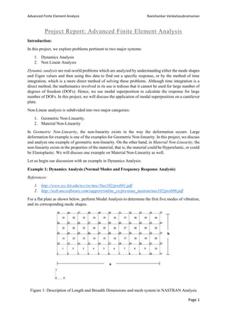
  • 1. Advanced Finite Element Analysis Ravishankar Venkatasubramanian Page 1 Project Report: Advanced Finite Element Analysis Introduction: In this project, we explore problems pertinent to two major systems: 1. Dynamics Analysis 2. Non Linear Analysis Dynamic analysis are real-world problems which are analyzed by understanding either the mode shapes and Eigen values and then using this data to find out a specific response, or by the method of time integration, which is a more direct method of solving these problems. Although time integration is a direct method, the mathematics involved in its use is tedious that it cannot be used for large number of degrees of freedom (DOFs). Hence, we use modal superposition to calculate the response for large number of DOFs. In this project, we will discuss the application of modal superposition on a cantilever plate. Non-Linear analysis is subdivided into two major categories: 1. Geometric Non-Linearity. 2. Material Non-Linearity In Geometric Non-Linearity, the non-linearity exists in the way the deformation occurs. Large deformation for example is one of the examples for Geometric Non-linearity. In this project, we discuss and analyze one example of geometric non-linearity. On the other hand, in Material Non-Linearity, the non-linearity exists in the properties of the material, that is, the material could be Hyperelastic, or could be Elastoplastic. We will discuss one example on Material Non-Linearity as well. Let us begin our discussion with an example in Dynamics Analysis: Example 1: Dynamics Analysis (Normal Modes and Frequency Response Analysis) References: 1. http://www.scc.kit.edu/scc/sw/msc/Nas102/prob01.pdf 2. http://web.mscsoftware.com/support/online_ex/previous_nastran/nas102/prob06.pdf For a flat plate as shown below, perform Modal Analysis to determine the first five modes of vibration, and its corresponding mode shapes. Figure 1: Description of Length and Breadth Dimensions and mesh system in NASTRAN Analysis
  • 2. Advanced Finite Element Analysis Ravishankar Venkatasubramanian Page 2 Figure 2: Material Properties The system is excited by a 0.1 psi pressure load over the total surface of the plate and a 1.0 lb. force at a corner of the tip lagging 45°. Use a modal damping of ξ = 0.03. Use a frequency step of 20 Hz between a range of 20Hz and 1000 Hz. Perform Modal Frequency Response analysis for the mentioned loads and boundary conditions: Figure 3: Boundary Conditions and Load Solution: We use ANSYS Workbench 17.0 for the analysis and simulation. The solution was first attempted using 3D- Hexahedral elements. The initial analysis to be done was Modal Analysis. A fixed support boundary condition is applied to the system, as shown in Figure 4.
  • 3. Advanced Finite Element Analysis Ravishankar Venkatasubramanian Page 3 Figure 4: Boundary Condition for Eigen Value Analysis After the boundary conditions are applied, the number of modes to be found are written in the Analysis settings tab, as shown in Figure 5: Figure 5: Analysis Settings – Modal Analysis After this step, Eigen value analysis is run to find out the Mode shapes (Eigen vectors) and Eigen Values (Natural Frequency), as shown in Figure 6 and Figure 7. Figure 6: Natural Frequency for each mode
  • 4. Advanced Finite Element Analysis Ravishankar Venkatasubramanian Page 4 Figure 7: Mode Shape 1 for a Natural Frequency of 131.79 Hz. These answers of fundamental frequencies from Figure 6 match closely with the answers obtained in the NASTRAN Example problem (from reference), as shown in Figure 8 (Natural Frequency circled in blue): Figure 8: Eigen Values and Natural Frequencies from NASTRAN Example Problem. Varying the mesh density and the type of element (From Hexahedral to Tetrahedral) gives tiny change in Modal Frequency, which is not highly significant. Using these Eigen Values, we now move on to Frequency Response Analysis. In frequency response analysis, we use the Eigen values to find out Frequency response as a function of these mode shapes and modal frequencies. This method saves a lot of time compared to the direct method. Figure 9 provides the geometry, and the requisite boundary conditions applied.
  • 5. Advanced Finite Element Analysis Ravishankar Venkatasubramanian Page 5 Figure 9: Boundary Conditions on the Model Initially, hexahedral elements are used for the analysis, and the mesh density is at its coarsest. This analysis is run with the mentioned damping ratio and the frequency range, with mentioned steps in frequency is taken, as shown in Figure 10. Figure 10: Analysis Settings
  • 6. Advanced Finite Element Analysis Ravishankar Venkatasubramanian Page 6 With the mentioned Analysis settings, the Frequency Response Analysis (FRA) was run. The FRA peaks are shown in Figure 11: Figure 11: FRA peaks for Hexahedral Elements The FRA peaks show that the displacement amplitude is highest near the resonance frequencies between 10Hz- 1000Hz. This is expected for the question as instability generally exists near the resonant frequencies. The value of displacement can be further refined by using a finer mesh. Testing has also been done using Tetrahedral mesh, and the displacement has been found to be close to the answer mentioned in the NASTRAN Manual (Figure 12) for fine Hexahedral mesh. Hexahedral elements have more nodes, and hence can handle bending better than Tetrahedral elements. A finer mesh provides closer interpolation values, and more accurate results. Figure 12: PATRAN Results from Reference for FRA
  • 7. Advanced Finite Element Analysis Ravishankar Venkatasubramanian Page 7 FRA analysis for higher number of solution intervals, i.e., higher number of frequencies between 20Hz- 1000Hz provides a smoother curve with higher accuracy of results. But these results cannot be compared with the results from Figure 12, which is based on a solution interval of 49. For Tetrahedral elements, the FRA provides a higher displacement, since the tetrahedral elements cannot handle bending and oscillatory movements as effectively as Hexahedral elements, there is a slightly higher displacement, as shown in Figure 13. Figure 13: FRA peaks for Tetrahedral Elements The system is a plate system, and cannot be modeled as a 1D system, and hence, we restrict its modeling. With increase in mesh density, there is an increase in accuracy. Hence, the most accurate mesh to use in this case is a Fine-Hexahedral mesh. Example 2: (Large Deformation; Geometric Non-Linearity) Reference: http://support.midasnfx.com/files/NAFEMS-PDF/Z-shaped%20cantilever.pdf Figure 14 shows a Z-shaped cantilever laid along the oblique line of 45˚. The total load P at all the points on the free end D in the positive Z-direction is conservative (non-follower load). The material properties are also given. Figure 14: Z- Shaped Cantilever
  • 8. Advanced Finite Element Analysis Ravishankar Venkatasubramanian Page 8 Solution: This system is designed on ANSYS Workbench 17.0 using the Design Modeler. The model was initially modeled as a 3D system, and later modeled as a 2D system and a 1D system. We will discuss about the results of each system in detail. Figure 15: Hexahedral Coarse Mesh Figure 16 shows details of the boundary conditions. The fixed support boundary condition and Force is applied in a ramped fashion, over a period of time. Figure 16: Boundary Conditions on the Z-Shaped Cantilever
  • 9. Advanced Finite Element Analysis Ravishankar Venkatasubramanian Page 9 Figure 17: Application of Ramped Force Ramped force is essential to make sure that the system does not collapse due to sudden application of forces up to 4000N. Figure 18: Analysis Settings The number of steps is set to 100 to obtain an accurate non-linear solution. The other controls are set to program controlled as the question does not mention any other specific changes to make to the system. The final deformation, at Load = 4000N is shown in Figure 19:
  • 10. Advanced Finite Element Analysis Ravishankar Venkatasubramanian Page 10 Figure 19: Directional Deformation of the system at 4000N Load A graph is drawn with displacement in the X-Axis and Load in the Y-axis, to get an idea about how the system deforms with increasing force. The displacement rapidly increases with load for the first 500N. After this force, the deformation has reached around 100mm, where the mid-section of the Z-shaped cantilever causes ‘tension stiffening’, as shown in Figure 20. This tension stiffening continues all the way upto the load of 4000N, and it can be see that there is very less displacement (43mm) over a large amount of force (3500N). This can be attributed solely to the stiffening in the mid-section of the Z shaped cantilever. Please note that the deformation shown in Figure 19 is only for the tip of the cantilever. Figure 20: Tip Displacement vs Load (Z Shaped Cantilever) This graph is compared with the graph obtained from the Midas-NFX reference, shown in Figure 20. 0 500 1000 1500 2000 2500 3000 3500 4000 4500 0 20 40 60 80 100 120 140 160 Load(N) Tip Displacement (mm) Tip Displacement vs Load
  • 11. Advanced Finite Element Analysis Ravishankar Venkatasubramanian Page 11 Figure 21: Tip Displacement vs Displacement (Midas-NFX) Comparing both Figure 20 and Figure 21, we can conclude that the graphs are almost the same. Increasing the mesh density in both 3D and 1D has not provided a significant increase in the accuracy of the system. This is probably because the system is well equipped to handle bending as such, and the slow increase in displacement due to tension stiffening has provided sufficient iterations to weed out any numerical errors, which might creep in the analysis. The 3D Hexahedral elements can handle bending effectively, and hence, provide accurate results. Figure 22, 23 show pictures of the final deformation in both 2D and 1D systems. Figure 22: Tip Deformation – Quadrilateral Shell Elements
  • 12. Advanced Finite Element Analysis Ravishankar Venkatasubramanian Page 12 Figure 23: Tip Deformation – 1D Beam Elements As seen from Figure 22, 1D beam elements can handle bending effectively, and hence, the deformation at the tip matches with 3D Tetrahedral/Hexahedral elements. 2D triangular and Quadrilateral elements on the other hand, cannot handle bending as effectively as beam elements, and provide slightly more deformation. This is seen in Figure 21. There is no significant change in tip displacement with mesh density, and hence, that has not been discussed in detail. For further information, the attached input files provide 3 different mesh densities, along with all element types (3D, 2D and 1D). The solution has been compared with the reference Midas-NFX, and has been found to match with the prescribed result. Example 3: (Material Non-Linearity: Elasto-Plastic Material) Reference: http://www.scc.kit.edu/scc/sw/msc/Nas103/Workshop_6.pdf Figure 24: Diagram of Problem L=50, W=10, T=0.1. The material used in this system has the following properties: Young’s Modulus = 3.0E+6, Poisson’s Ratio = 0.25, Tangent Modulus = 30303, Yield Stress = 850.
  • 13. Advanced Finite Element Analysis Ravishankar Venkatasubramanian Page 13 Find the Elastic and Plastic Strain at the end of the loading. The loading cycle is: 1. Load P=800 2. Load P= 1000 3. Unload P= 950 4. Unload P=0 Solution: The modeling can be done by using a quarter of the model (symmetry), and it will yield the same result with a lesser time duration involved. But for this problem, we use a system which has the entire bar. Figure 25 shows the meshed bar, with a coarse hexahedral mesh. Figure 25: Meshed Part – Hexahedral Mesh We expect, from the loading pattern that the material yields between 1 and 2 seconds, since the Yield stress is 850. After yielding, the material will maintain its plastic nature, even if it unloads, as done in t=3 and t=4. The loading history is shown in Figure 26 (This is because the stress is F/A=Load/(10*0.1)=> Stress = Load). Figure 26: Load curve with time
  • 14. Advanced Finite Element Analysis Ravishankar Venkatasubramanian Page 14 The boundary conditions applied on the system are shown in Figure 27. Figure 27: Application of Boundary Conditions The analysis is run, and the requested outputs are equivalent plastic strain, the total strain in the body and the equivalent von-mises stress. The analysis is run under these conditions. Applying a fixed boundary condition on one end provides a system which is constrained, and the simulation can proceed as expected. The system is the same as the one where the tensile load is applied to both ends. The equivalent plastic strain is shown in Figure 28: Figure 28: Equivalent Plastic Strain in the system at t=4s (Final) The system shows an equivalent plastic strain of 5.73mm, which is the same as plastic strain obtained when the load is 1000.
  • 15. Advanced Finite Element Analysis Ravishankar Venkatasubramanian Page 15 The graph between time and equivalent plastic strain is: Figure 29: Plastic Strain vs Time The plastic strain remains constant in unloading, as expected, as all the elastic strain is dissipated in unloading. The graph between time and Equivalent total strain is: Figure 30: Total Strain vs Time The total strain reduces over time in the unloading process as the elastic strain is dissipated over time during the unloading procedure. Now, we can draw a graph between the equivalent stress and plastic strain. Figure 31: Plastic Strain and Equivalent Stress 0 200 400 600 800 1000 1200 -0.001 0 0.001 0.002 0.003 0.004 0.005 0.006 0.007 Plastic Strain vs Equivalent Stress Plastic Strain vs Equivalent Stress
  • 16. Advanced Finite Element Analysis Ravishankar Venkatasubramanian Page 16 This graph can now be compared with Figure 32, which is the graph between Plastic Strain and Equivalent stress in the reference: Figure 32: Plastic Strain vs Stress (Reference Material) As seen in this system, we can say that the solution is an almost perfect match. Increasing the mesh density provides more accuracy in the system, but changing the element type from 3D to 2D will not cause much improvement in results. This is because Hexahedral or any element in the 3D domain can handle stretching efficiently. Hence, this system can be meshed with any element, 3D, 2D or 1D to get effective results.