Download as PDF, PPTX


![Experiments using R
juul2 data frame in the ISwR package contains insulin-like growth
factor, one observation per subject in various ages, with the bulk of
the data collected in conection with physical examinations.
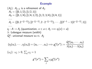
n = 1336
setClass("random.variable", representation(data="numeric",
breaks="array",width="array"))
setClass("continuous", contains="random.variable",
representation(mu="numeric",sigma="numeric"))
setClass("discrete", contains="random.variable")
X[[1]]<-new("continuous", data=juul2$age)
X[[2]]<-new("continuous", data=juul2$height)
X[[3]]<-new("discrete", data=juul2$menarche)
X[[4]]<-new("discrete", data=juul2$sex)
X[[5]]<-new("discrete", data=juul2$igf1)
X[[6]]<-new("discrete", data=juul2$tanner)
X[[7]]<-new("discrete", data=juul2$testvol)
X[[8]]<-new("continuous", data=juul2$weight)](https://image.slidesharecdn.com/2013-10-27-170405223602/85/The-Universal-Bayesian-Chow-Liu-Algorithm-15-320.jpg)
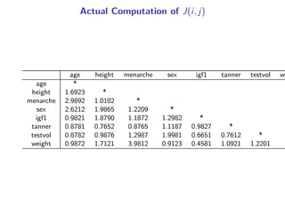


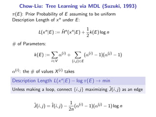
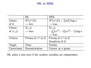
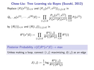
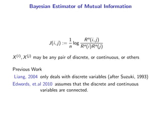
The Universal Bayesian Chow-Liu Algorithm summarizes a document describing a method for learning Bayesian networks from data that can contain both discrete and continuous variables. It constructs a tree structure that maximizes the posterior probability based on estimating mutual information between all variable pairs. The algorithm was tested on real world medical data containing different variable types. Future work includes developing an R command to implement the full algorithm.


![Polymer [ बहुलक ] Chemistry Notes PDF - Irfanullah Mehar - JJ Sir Chemistry.pdf](https://cdn.slidesharecdn.com/ss_thumbnails/polymerchemistrynotespdf-irfanullahmehar-jjsirchemistry-260210172118-3f9b37f7-thumbnail.jpg?width=640&height=640&fit=bounds)


![ANIMAL_CELL_,_TISSUE_AND_ORGAN_CULTURE[1].pptx](https://cdn.slidesharecdn.com/ss_thumbnails/animalcelltissueandorganculture1-260204172026-4462b440-thumbnail.jpg?width=640&height=640&fit=bounds)


