1. Integrating Functions of Time

x
1 2 3 4 t

2. Integrating Functions of Time

x
4
change in displacement   xdt

0
1 2 3 4 t

3. Integrating Functions of Time

x
4
change in displacement   xdt

0
1 2 3 4 t 1 3 4
change in distance   xdt   xdt   xdt
  
0 1 3

4. Integrating Functions of Time

x
4
change in displacement   xdt

0
1 2 3 4 t 1 3 4
change in distance   xdt   xdt   xdt
  
0 1 3

x
1 2 3 4 t

5. Integrating Functions of Time

x
4
change in displacement   xdt

0
1 2 3 4 t 1 3 4
change in distance   xdt   xdt   xdt
  
0 1 3

x
4
change in velocity   dt
x
0
1 2 3 4 t

6. Integrating Functions of Time

x
4
change in displacement   xdt

0
1 2 3 4 t 1 3 4
change in distance   xdt   xdt   xdt
  
0 1 3

x
4
change in velocity   dt
x
0
1 2 3 4 t 2 4
change in speed    dt   dt
x x
0 2

7. Derivative Graphs
Function 1st derivative 2nd derivative
displacement velocity acceleration

8. Derivative Graphs
Function 1st derivative 2nd derivative
displacement velocity acceleration
stationary point x intercept

9. Derivative Graphs
Function 1st derivative 2nd derivative
displacement velocity acceleration
stationary point x intercept
inflection point stationary point x intercept

10. Derivative Graphs
Function 1st derivative 2nd derivative
displacement velocity acceleration
stationary point x intercept
inflection point stationary point x intercept
increasing positive

11. Derivative Graphs
Function 1st derivative 2nd derivative
displacement velocity acceleration
stationary point x intercept
inflection point stationary point x intercept
increasing positive
decreasing negative

12. Derivative Graphs
Function 1st derivative 2nd derivative
displacement velocity acceleration
stationary point x intercept
inflection point stationary point x intercept
increasing positive
decreasing negative
concave up increasing positive

13. Derivative Graphs
Function 1st derivative 2nd derivative
displacement velocity acceleration
stationary point x intercept
inflection point stationary point x intercept
increasing positive
decreasing negative
concave up increasing positive
concave down decreasing negative

14. graph type integrate differentiate

15. graph type integrate differentiate
horizontal line oblique line x axis

16. graph type integrate differentiate
horizontal line oblique line x axis
oblique line parabola horizontal line

17. graph type integrate differentiate
horizontal line oblique line x axis
oblique line parabola horizontal line
parabola cubic oblique line
inflects at turning pt

18. graph type integrate differentiate
horizontal line oblique line x axis
oblique line parabola horizontal line
parabola cubic oblique line
inflects at turning pt
Remember:
• integration = area

19. graph type integrate differentiate
horizontal line oblique line x axis
oblique line parabola horizontal line
parabola cubic oblique line
inflects at turning pt
Remember:
• integration = area
• on a velocity graph, total area = distance
total integral = displacement

20. graph type integrate differentiate
horizontal line oblique line x axis
oblique line parabola horizontal line
parabola cubic oblique line
inflects at turning pt
Remember:
• integration = area
• on a velocity graph, total area = distance
total integral = displacement
• on an acceleration graph, total area = speed
total integral = velocity

21. (ii) 2003 HSC Question 7b)
The velocity of a particle is given by v  2  4 cos t for 0  t  2 ,
where v is measured in metres per second and t is measured in seconds
(i) At what times during this period is the particle at rest?

22. (ii) 2003 HSC Question 7b)
The velocity of a particle is given by v  2  4 cos t for 0  t  2 ,
where v is measured in metres per second and t is measured in seconds
(i) At what times during this period is the particle at rest?
v0
2  4cos t  0
1
cos t 
2

23. (ii) 2003 HSC Question 7b)
The velocity of a particle is given by v  2  4 cos t for 0  t  2 ,
where v is measured in metres per second and t is measured in seconds
(i) At what times during this period is the particle at rest?
v0 Q1, 4
2  4cos t  0 1
1 cos  
cos t  2
2 

3

24. (ii) 2003 HSC Question 7b)
The velocity of a particle is given by v  2  4 cos t for 0  t  2 ,
where v is measured in metres per second and t is measured in seconds
(i) At what times during this period is the particle at rest?
v0 Q1, 4 t   , 2  
2  4cos t  0 1  5
1 cos   t ,
cos t  2 3 3
2 

3
 5
 particle is at rest after seconds and again after seconds
3 3

25. (ii) 2003 HSC Question 7b)
The velocity of a particle is given by v  2  4 cos t for 0  t  2 ,
where v is measured in metres per second and t is measured in seconds
(i) At what times during this period is the particle at rest?
v0 Q1, 4 t   , 2  
2  4cos t  0 1  5
1 cos   t ,
cos t  2 3 3
2 

3
 5
 particle is at rest after seconds and again after seconds
3 3
(ii) What is the maximum velocity of the particle during this period?

26. (ii) 2003 HSC Question 7b)
The velocity of a particle is given by v  2  4 cos t for 0  t  2 ,
where v is measured in metres per second and t is measured in seconds
(i) At what times during this period is the particle at rest?
v0 Q1, 4 t   , 2  
2  4cos t  0 1  5
1 cos   t ,
cos t  2 3 3
2 

3
 5
 particle is at rest after seconds and again after seconds
3 3
(ii) What is the maximum velocity of the particle during this period?
4  4 cos t  4
2  2  4 cos t  6
 maximum velocity is 6 m/s

27. (iii) Sketch the graph of v as a function of t for 0  t  2

28. (iii) Sketch the graph of v as a function of t for 0  t  2
2 2
amplitude  4 units period  divisions 
shift  2 units 1 4
 2 
flip upside down 
2

29. (iii) Sketch the graph of v as a function of t for 0  t  2
2 2
amplitude  4 units period  divisions 
shift  2 units 1 4
 2 
flip upside down 
2
v
6
5
4
3
2
1
-1
  3 2 t
-2
2 2

30. (iii) Sketch the graph of v as a function of t for 0  t  2
2 2
amplitude  4 units period  divisions 
shift  2 units 1 4
 2 
flip upside down 
2
v
6
5
4
3
2
1
-1
  3 2 t
-2
2 2

31. (iii) Sketch the graph of v as a function of t for 0  t  2
2 2
amplitude  4 units period  divisions 
shift  2 units 1 4
 2 
flip upside down 
2
v
6
5
4
3
2
1
-1
  3 2 t
-2
2 2

32. (iii) Sketch the graph of v as a function of t for 0  t  2
2 2
amplitude  4 units period  divisions 
shift  2 units 1 4
 2 
flip upside down 
2
v
6
5
4
3
2
1
-1
  3 2 t
-2
2 2

33. (iii) Sketch the graph of v as a function of t for 0  t  2
2 2
amplitude  4 units period  divisions 
shift  2 units 1 4
 2 
flip upside down 
2
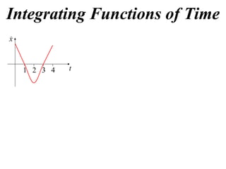
v
6
5 v  2  4 cos t
4
3
2
1
-1
  3 2 t
-2
2 2

34. (iv) Calculate the total distance travelled by the particle between t = 0
and t = 

35. (iv) Calculate the total distance travelled by the particle between t = 0
and t = 

3 
distance =    2  4 cos t  dt    2  4 cos t  dt
0 
3

36. (iv) Calculate the total distance travelled by the particle between t = 0
and t = 

3 
distance =    2  4 cos t  dt    2  4 cos t  dt
0 
=  2t  4sin t    2t 3 4sin t 
0 
3 3

37. (iv) Calculate the total distance travelled by the particle between t = 0
and t = 

3 
distance =    2  4 cos t  dt    2  4 cos t  dt
0 
=  2t  4sin t    2t 3 4sin t 
0 
3 3
 2  4sin  
=  0  0    2  4sin    2  
 3 3
 2 4 3 
=2  2   
 3 2 
2
=4 3  metres
3

38. (iii) 2004 HSC Question 9b)
A particle moves along the x-axis. Initially it is at rest at the origin.
The graph shows the acceleration, a, of the particle as a function of
time t for 0  t  5
(i) Write down the time at which the velocity of the particle is a maximum

39. (iii) 2004 HSC Question 9b)
A particle moves along the x-axis. Initially it is at rest at the origin.
The graph shows the acceleration, a, of the particle as a function of
time t for 0  t  5
(i) Write down the time at which the velocity of the particle is a maximum
v   adt
 adt is a maximum when t  2

40. (iii) 2004 HSC Question 9b)
A particle moves along the x-axis. Initially it is at rest at the origin.
The graph shows the acceleration, a, of the particle as a function of
time t for 0  t  5
(i) Write down the time at which the velocity of the particle is a maximum
dv
v   adt OR v is a maximum when 0
dt
 adt is a maximum when t  2

41. (iii) 2004 HSC Question 9b)
A particle moves along the x-axis. Initially it is at rest at the origin.
The graph shows the acceleration, a, of the particle as a function of
time t for 0  t  5
(i) Write down the time at which the velocity of the particle is a maximum
dv
v   adt OR v is a maximum when 0
dt
 adt is a maximum when t  2
 velocity is a maximum when t  2 seconds

42. (ii) At what time during the interval 0  t  5 is the particle furthest
from the origin? Give reasons for your answer.

43. (ii) At what time during the interval 0  t  5 is the particle furthest
from the origin? Give reasons for your answer.
Question is asking, “when is displacement a maximum?”
dx
x is a maximum when 0
dt

44. (ii) At what time during the interval 0  t  5 is the particle furthest
from the origin? Give reasons for your answer.
Question is asking, “when is displacement a maximum?”
dx
x is a maximum when 0
dt
But v   adt
 We must solve  adt  0

45. (ii) At what time during the interval 0  t  5 is the particle furthest
from the origin? Give reasons for your answer.
Question is asking, “when is displacement a maximum?”
dx
x is a maximum when 0
dt
But v   adt
 We must solve  adt  0
i.e. when is area above the axis = area below
By symmetry this would be at t = 4
 particle is furthest from the origin at t  4 seconds

46. (iv) 2007 HSC Question 10a) dx
An object is moving on the x-axis. The graph shows the velocity, ,
dt
of the object, as a function of t.
The coordinates of the points shown on the graph are A(2,1), B(4,5),
C(5,0) and D(6,–5). The velocity is constant for t  6
(i) Using Simpson’s rule, estimate the distance travelled between t = 0
and t = 4

47. (iv) 2007 HSC Question 10a) dx
An object is moving on the x-axis. The graph shows the velocity, ,
dt
of the object, as a function of t.
The coordinates of the points shown on the graph are A(2,1), B(4,5),
C(5,0) and D(6,–5). The velocity is constant for t  6
(i) Using Simpson’s rule, estimate the distance travelled between t = 0
and t = 4 h
distance   y0  4 yodd  2 yeven  yn 
3

48. (iv) 2007 HSC Question 10a) dx
An object is moving on the x-axis. The graph shows the velocity, ,
dt
of the object, as a function of t.
The coordinates of the points shown on the graph are A(2,1), B(4,5),
C(5,0) and D(6,–5). The velocity is constant for t  6
(i) Using Simpson’s rule, estimate the distance travelled between t = 0
and t = 4 h
distance   y0  4 yodd  2 yeven  yn 
3
t 0 2 4
v 0 1 5

49. (iv) 2007 HSC Question 10a) dx
An object is moving on the x-axis. The graph shows the velocity, ,
dt
of the object, as a function of t.
The coordinates of the points shown on the graph are A(2,1), B(4,5),
C(5,0) and D(6,–5). The velocity is constant for t  6
(i) Using Simpson’s rule, estimate the distance travelled between t = 0
and t = 4 h
distance   y0  4 yodd  2 yeven  yn 
3
1 4 1
t 0 2 4
v 0 1 5

50. (iv) 2007 HSC Question 10a) dx
An object is moving on the x-axis. The graph shows the velocity, ,
dt
of the object, as a function of t.
The coordinates of the points shown on the graph are A(2,1), B(4,5),
C(5,0) and D(6,–5). The velocity is constant for t  6
(i) Using Simpson’s rule, estimate the distance travelled between t = 0
and t = 4 h
distance   y0  4 yodd  2 yeven  yn 
3
1 4 1 2
 0  4 1  5
t 0 2 4 3
v 0 1 5
 6 metres

51. (ii) The object is initially at the origin. During which time(s) is the
displacement decreasing?

52. (ii) The object is initially at the origin. During which time(s) is the
displacement decreasing?
dx
x is decreasing when 0
dt
 displacement is decreasing when t  5 seconds

53. (ii) The object is initially at the origin. During which time(s) is the
displacement decreasing?
dx
x is decreasing when 0
dt
 displacement is decreasing when t  5 seconds
(iii) Estimate the time at which the object returns to the origin. Justify
your answer.

54. (ii) The object is initially at the origin. During which time(s) is the
displacement decreasing?
dx
x is decreasing when 0
dt
 displacement is decreasing when t  5 seconds
(iii) Estimate the time at which the object returns to the origin. Justify
your answer.
Question is asking, “when is displacement = 0?”

55. (ii) The object is initially at the origin. During which time(s) is the
displacement decreasing?
dx
x is decreasing when 0
dt
 displacement is decreasing when t  5 seconds
(iii) Estimate the time at which the object returns to the origin. Justify
your answer.
Question is asking, “when is displacement = 0?”
But x   vdt
 We must solve  vdt  0

56. (ii) The object is initially at the origin. During which time(s) is the
displacement decreasing?
dx
x is decreasing when 0
dt
 displacement is decreasing when t  5 seconds
(iii) Estimate the time at which the object returns to the origin. Justify
your answer.
Question is asking, “when is displacement = 0?”
But x   vdt
 We must solve  vdt  0
i.e. when is area above the axis = area below

57. (ii) The object is initially at the origin. During which time(s) is the
displacement decreasing?
dx
x is decreasing when 0
dt
 displacement is decreasing when t  5 seconds
(iii) Estimate the time at which the object returns to the origin. Justify
your answer.
Question is asking, “when is displacement = 0?”
But x   vdt
 We must solve  vdt  0
i.e. when is area above the axis = area below
By symmetry, area from t = 4 to 5 equals area
from t = 5 to 6

58. (ii) The object is initially at the origin. During which time(s) is the
displacement decreasing?
dx
x is decreasing when 0
dt
 displacement is decreasing when t  5 seconds
(iii) Estimate the time at which the object returns to the origin. Justify
your answer.
Question is asking, “when is displacement = 0?”
But x   vdt
 We must solve  vdt  0
i.e. when is area above the axis = area below
By symmetry, area from t = 4 to 5 equals area
from t = 5 to 6
In part (i) we estimated area from t = 0 to 4 to be 6,

59. (ii) The object is initially at the origin. During which time(s) is the
displacement decreasing?
dx
x is decreasing when 0
dt
 displacement is decreasing when t  5 seconds
(iii) Estimate the time at which the object returns to the origin. Justify
your answer.
Question is asking, “when is displacement = 0?”
But x   vdt
 We must solve  vdt  0
i.e. when is area above the axis = area below
By symmetry, area from t = 4 to 5 equals area A4
from t = 5 to 6
In part (i) we estimated area from t = 0 to 4 to be 6,
 A4  6

60. (ii) The object is initially at the origin. During which time(s) is the
displacement decreasing?
dx
x is decreasing when 0
dt
 displacement is decreasing when t  5 seconds
(iii) Estimate the time at which the object returns to the origin. Justify
your answer.
Question is asking, “when is displacement = 0?”
But x   vdt
 We must solve  vdt  0
a
i.e. when is area above the axis = area below
By symmetry, area from t = 4 to 5 equals area A4 5
from t = 5 to 6
In part (i) we estimated area from t = 0 to 4 to be 6,
 A4  6 a  1.2
5a  6

61. (ii) The object is initially at the origin. During which time(s) is the
displacement decreasing?
dx
x is decreasing when 0
dt
 displacement is decreasing when t  5 seconds
(iii) Estimate the time at which the object returns to the origin. Justify
your answer.
Question is asking, “when is displacement = 0?”
But x   vdt
 We must solve  vdt  0
a
i.e. when is area above the axis = area below
By symmetry, area from t = 4 to 5 equals area A4 5
from t = 5 to 6
In part (i) we estimated area from t = 0 to 4 to be 6,
 A4  6 a  1.2
5a  6  particle returns to the origin when t  7.2 seconds

62. (iv) Sketch the displacement, x, as a function of time.

63. (iv) Sketch the displacement, x, as a function of time.
x
8.5
6
2 4 6 8 t

64. (iv) Sketch the displacement, x, as a function of time.
object is initially at the origin
x
8.5
6
2 4 6 8 t

65. (iv) Sketch the displacement, x, as a function of time.
object is initially at the origin
when t = 4, x = 6
x
8.5
6
2 4 6 8 t

66. (iv) Sketch the displacement, x, as a function of time.
object is initially at the origin
when t = 4, x = 6
by symmetry of areas t = 6, x = 6
x
8.5
6
2 4 6 8 t

67. (iv) Sketch the displacement, x, as a function of time.
object is initially at the origin
when t = 4, x = 6
by symmetry of areas t = 6, x = 6
Area of triangle = 2.5
 when t  5, x  8.5
x
8.5
6
2 4 6 8 t

68. (iv) Sketch the displacement, x, as a function of time.
object is initially at the origin
when t = 4, x = 6
by symmetry of areas t = 6, x = 6
Area of triangle = 2.5
 when t  5, x  8.5
returns to x = 0 when t = 7.2
x
8.5
6
2 4 6 7.2 8 t

69. (iv) Sketch the displacement, x, as a function of time.
object is initially at the origin
when t = 4, x = 6
by symmetry of areas t = 6, x = 6
Area of triangle = 2.5
 when t  5, x  8.5
returns to x = 0 when t = 7.2
x
v is steeper between t = 2 and 4
8.5
than between t = 0 and 2
6  particle covers more distance
between t  2 and 4
2 4 6 7.2 8 t

70. (iv) Sketch the displacement, x, as a function of time.
object is initially at the origin
when t = 4, x = 6
by symmetry of areas t = 6, x = 6
Area of triangle = 2.5
 when t  5, x  8.5
returns to x = 0 when t = 7.2
x
v is steeper between t = 2 and 4
8.5
than between t = 0 and 2
6  particle covers more distance
between t  2 and 4
when t > 6, v is constant
t  when t  6, x is a straight line
2 4 6 7.2 8

71. (iv) Sketch the displacement, x, as a function of time.
object is initially at the origin
when t = 4, x = 6
by symmetry of areas t = 6, x = 6
Area of triangle = 2.5
 when t  5, x  8.5
returns to x = 0 when t = 7.2
x
v is steeper between t = 2 and 4
8.5
than between t = 0 and 2
6  particle covers more distance
between t  2 and 4
when t > 6, v is constant
t  when t  6, x is a straight line
2 4 6 7.2 8

72. (v) 2005 HSC Question 7b)
dx
The graph shows the velocity, dt , of a particle as a function of time.
Initially the particle is at the origin.
(i) At what time is the displacement, x, from the origin a maximum?

73. (v) 2005 HSC Question 7b)
dx
The graph shows the velocity, dt , of a particle as a function of time.
Initially the particle is at the origin.
(i) At what time is the displacement, x, from the origin a maximum?
Displacement is a maximum when area is most positive, also when
velocity is zero
i.e. when t = 2

74. (ii) At what time does the particle return to the origin? Justify
your answer

75. (ii) At what time does the particle return to the origin? Justify
your answer
Question is asking, “when is displacement = 0?”
i.e. when is area above the axis = area below?

76. (ii) At what time does the particle return to the origin? Justify
your answer
2 a w
a 2
Question is asking, “when is displacement = 0?”
i.e. when is area above the axis = area below?

77. (ii) At what time does the particle return to the origin? Justify
your answer
2 a w
a 2
Question is asking, “when is displacement = 0?”
i.e. when is area above the axis = area below?
2w = 2
w=1

78. (ii) At what time does the particle return to the origin? Justify
your answer
2 a w
a 2
Question is asking, “when is displacement = 0?”
i.e. when is area above the axis = area below?
2w = 2
w=1
Returns to the origin after 4 seconds

79. d 2x
(iii) Draw a sketch of the acceleration, 2 , as afunction of
dt
time for 0  t  6
d 2x
dt 2
1 2 3 5 6 t

80. d 2x
(iii) Draw a sketch of the acceleration, 2 , as afunction of
dt
time for 0  t  6 differentiate a horizontal line
you get the xaxis
d 2x
dt 2
1 2 3 5 6 t

81. d 2x
(iii) Draw a sketch of the acceleration, 2 , as afunction of
dt
time for 0  t  6 differentiate a horizontal line
you get the xaxis
from 1 to 3 we have a cubic,
inflects at 2, and is decreasing
differentiate, you get a parabola,
stationary at 2, it is below the x axis
d 2x
dt 2
1 2 3 5 6 t

82. d 2x
(iii) Draw a sketch of the acceleration, 2 , as afunction of
dt
time for 0  t  6 differentiate a horizontal line
you get the xaxis
from 1 to 3 we have a cubic,
inflects at 2, and is decreasing
differentiate, you get a parabola,
stationary at 2, it is below the x axis
d 2x
dt 2
from 5 to 6 is a cubic, inflects at 6
and is increasing (using symmetry)
differentiate, you get a parabola
1 2 3 5 6 t
stationary at 6, it is above the x axis

83. d 2x
(iii) Draw a sketch of the acceleration, 2 , as afunction of
dt
time for 0  t  6 differentiate a horizontal line
you get the xaxis
from 1 to 3 we have a cubic,
inflects at 2, and is decreasing
differentiate, you get a parabola,
stationary at 2, it is below the x axis
d 2x
dt 2
from 5 to 6 is a cubic, inflects at 6
and is increasing (using symmetry)
differentiate, you get a parabola
1 2 3 5 6 t
stationary at 6, it is above the x axis

84. Exercise 3C; 1 ace etc, 2 ace etc, 4a, 7ab(i), 8, 9a, 10, 13, 15, 16, 18