inverse trig functions and linear trig equations

1. –π/2
π/2
The Graphs of Inverse Trig–Functions
π
0
π/2
–π/2
π
0

2. Inverse Functions
Start with a calculator demos of sine & sine inverse
For the choice of the range.

3. A function f(x) = y takes an input x and produces
one output y.
Inverse Functions

4. A function f(x) = y takes an input x and produces
one output y. Often we represent a function by the
following figure.
Inverse Functions
domian rangex y=f(x)
f

5. A function f(x) = y takes an input x and produces
one output y. Often we represent a function by the
following figure.
Inverse Functions
We like to reverse the operation, i.e., if we know
the output y, what was (were) the input x?
domian rangex y=f(x)
f

6. A function f(x) = y takes an input x and produces
one output y. Often we represent a function by the
following figure.
Inverse Functions
We like to reverse the operation, i.e., if we know
the output y, what was (were) the input x?
This procedure of associating the output y to the
input x may or may not be a function.
domian rangex y=f(x)
f

7. A function f(x) = y takes an input x and produces
one output y. Often we represent a function by the
following figure.
Inverse Functions
We like to reverse the operation, i.e., if we know
the output y, what was (were) the input x?
This procedure of associating the output y to the
input x may or may not be a function.
domian rangex y=f(x)
f
If it is a function, it is called
the inverse function of f(x)
and it is denoted as f –1(y).

8. A function f(x) = y takes an input x and produces
one output y. Often we represent a function by the
following figure.
Inverse Functions
We like to reverse the operation, i.e., if we know
the output y, what was (were) the input x?
This procedure of associating the output y to the
input x may or may not be a function.
domian rangex y=f(x)
f
If it is a function, it is called
the inverse function of f(x)
and it is denoted as f –1(y).
x y=f(x)
f

9. A function f(x) = y takes an input x and produces
one output y. Often we represent a function by the
following figure.
Inverse Functions
We like to reverse the operation, i.e., if we know
the output y, what was (were) the input x?
This procedure of associating the output y to the
input x may or may not be a function.
domian rangex y=f(x)
f
If it is a function, it is called
the inverse function of f(x)
and it is denoted as f –1(y).
x=f–1(y) y=f(x)
f
f –1

10. A function f(x) = y takes an input x and produces
one output y. Often we represent a function by the
following figure.
Inverse Functions
We like to reverse the operation, i.e., if we know
the output y, what was (were) the input x?
This procedure of associating the output y to the
input x may or may not be a function.
domian rangex y=f(x)
f
If it is a function, it is called
the inverse function of f(x)
and it is denoted as f –1(y).
We say f(x) and f –1(y) are
the inverse of each other.
x=f–1(y) y=f(x)
f
f –1

11. Example A.
a. The function y = f(x) = 2x takes the input x and
doubles it to get the output y.
Inverse Functions

12. Example A.
a. The function y = f(x) = 2x takes the input x and
doubles it to get the output y. To reverse the
operation, take an output y,
Inverse Functions

13. Example A.
a. The function y = f(x) = 2x takes the input x and
doubles it to get the output y. To reverse the
operation, take an output y, divided it by 2 and we
get back to the x.
Inverse Functions

14. Example A.
a. The function y = f(x) = 2x takes the input x and
doubles it to get the output y. To reverse the
operation, take an output y, divided it by 2 and we
get back to the x. In other words f –1(y) = y/2.
Inverse Functions

15. Example A.
a. The function y = f(x) = 2x takes the input x and
doubles it to get the output y. To reverse the
operation, take an output y, divided it by 2 and we
get back to the x. In other words f –1(y) = y/2.
So, for example, f –1(6) = 3 because f(3) = 6.
Inverse Functions

16. Example A.
a. The function y = f(x) = 2x takes the input x and
doubles it to get the output y. To reverse the
operation, take an output y, divided it by 2 and we
get back to the x. In other words f –1(y) = y/2.
So, for example, f –1(6) = 3 because f(3) = 6.
b. Given y = f(x) = x2 and y = 9,
Inverse Functions

17. Example A.
a. The function y = f(x) = 2x takes the input x and
doubles it to get the output y. To reverse the
operation, take an output y, divided it by 2 and we
get back to the x. In other words f –1(y) = y/2.
So, for example, f –1(6) = 3 because f(3) = 6.
b. Given y = f(x) = x2 and y = 9, there are two inputs
namely x = 3 and x = –3 that give the output 9.
x=3
y=9
f(x)=x2
x=–3
Inverse Functions

18. Example A.
a. The function y = f(x) = 2x takes the input x and
doubles it to get the output y. To reverse the
operation, take an output y, divided it by 2 and we
get back to the x. In other words f –1(y) = y/2.
So, for example, f –1(6) = 3 because f(3) = 6.
b. Given y = f(x) = x2 and y = 9, there are two inputs
namely x = 3 and x = –3 that give the output 9.
Therefore, the reverse procedure is not a function
x=3
y=9
f(x)=x2
x=–3
not a function
Inverse Functions

19. Example A.
a. The function y = f(x) = 2x takes the input x and
doubles it to get the output y. To reverse the
operation, take an output y, divided it by 2 and we
get back to the x. In other words f –1(y) = y/2.
So, for example, f –1(6) = 3 because f(3) = 6.
b. Given y = f(x) = x2 and y = 9, there are two inputs
namely x = 3 and x = –3 that give the output 9.
Therefore, the reverse procedure is not a function
Inverse Functions
x=3
y=9
f(x)=x2
x=–3
not a function
Unless we intentionally select an
answer, f –1(9) is not well defined
Because there are two choices.

20. Example A.
a. The function y = f(x) = 2x takes the input x and
doubles it to get the output y. To reverse the
operation, take an output y, divided it by 2 and we
get back to the x. In other words f –1(y) = y/2.
So, for example, f –1(6) = 3 because f(3) = 6.
b. Given y = f(x) = x2 and y = 9, there are two inputs
namely x = 3 and x = –3 that give the output 9.
Therefore, the reverse procedure is not a function
so f –1(y) does not exist.
Inverse Functions
x=3
y=9
f(x)=x2
x=–3
not a function
Unless we intentionally select an
answer, f –1(9) is not well defined
Because there are two choices.

21. Example A.
a. The function y = f(x) = 2x takes the input x and
doubles it to get the output y. To reverse the
operation, take an output y, divided it by 2 and we
get back to the x. In other words f –1(y) = y/2.
So, for example, f –1(6) = 3 because f(3) = 6.
b. Given y = f(x) = x2 and y = 9, there are two inputs
namely x = 3 and x = –3 that give the output 9.
Therefore, the reverse procedure is not a function
so f –1(y) does not exist.
Inverse Functions
But g –1(y) exists for
y = g(x) = x2 with x ≥ 0,
and that g –1(9) = 3. In fact g –1(y) = √y.
x=3
y=9
f(x)=x2
x=–3
not a function

22. Example A.
a. The function y = f(x) = 2x takes the input x and
doubles it to get the output y. To reverse the
operation, take an output y, divided it by 2 and we
get back to the x. In other words f –1(y) = y/2.
So, for example, f –1(6) = 3 because f(3) = 6.
b. Given y = f(x) = x2 and y = 9, there are two inputs
namely x = 3 and x = –3 that give the output 9.
Therefore, the reverse procedure is not a function
so f –1(y) does not exist.
Inverse Functions
But g –1(y) exists for
y = g(x) = x2 with x ≥ 0,
and that g –1(9) = 3. In fact g –1(y) = √y. Hence the
existence of the inverse depends on the domain.
x=3
y=9
f(x)=x2
x=–3
not a function

23. Inverse Functions
u
v
u = v
a one-to-one function
A function is one-to-one if different inputs produce
different outputs or that two inputs give two outputs.

24. Inverse Functions
A function is one-to-one if different inputs produce
different outputs or that two inputs give two outputs.
That is, f(x) is said to be one-to-one if for every two
inputs u and v such that u  v, then f(u)  f(v).

25. Inverse Functions
u
v
u = v
a one-to-one function
A function is one-to-one if different inputs produce
different outputs or that two inputs give two outputs.
That is, f(x) is said to be one-to-one if for every two
inputs u and v such that u  v, then f(u)  f(v).

26. Inverse Functions
u f(u)
v f(v)
u = v f(u) = f(v)
a one-to-one function
A function is one-to-one if different inputs produce
different outputs or that two inputs give two outputs.
That is, f(x) is said to be one-to-one if for every two
inputs u and v such that u  v, then f(u)  f(v).

27. Inverse Functions
u f(u)
v f(v)
u = v f(u) = f(v)
a one-to-one function
u
v
u = v
not a one-to-one function
A function is one-to-one if different inputs produce
different outputs or that two inputs give two outputs.
That is, f(x) is said to be one-to-one if for every two
inputs u and v such that u  v, then f(u)  f(v).

28. Inverse Functions
u f(u)
v f(v)
u = v f(u) = f(v)
a one-to-one function
u
f(u)=f(v)
v
u = v
not a one-to-one function
A function is one-to-one if different inputs produce
different outputs or that two inputs give two outputs.
That is, f(x) is said to be one-to-one if for every two
inputs u and v such that u  v, then f(u)  f(v).

29. Example B.
a. g(x) = 2x is one-to-one
Inverse Functions
u f(u)
v f(v)
u = v f(u) = f(v)
a one-to-one function
u
f(u)=f(v)
v
u = v
not a one-to-one function
A function is one-to-one if different inputs produce
different outputs or that two inputs give two outputs.
That is, f(x) is said to be one-to-one if for every two
inputs u and v such that u  v, then f(u)  f(v).

30. Example B.
a. g(x) = 2x is one-to-one
because if u  v, then 2u  2v.
Inverse Functions
u f(u)
v f(v)
u = v f(u) = f(v)
a one-to-one function
u
f(u)=f(v)
v
u = v
not a one-to-one function
A function is one-to-one if different inputs produce
different outputs or that two inputs give two outputs.
That is, f(x) is said to be one-to-one if for every two
inputs u and v such that u  v, then f(u)  f(v).

31. Example B.
a. g(x) = 2x is one-to-one
because if u  v, then 2u  2v.
b. f(x) = x2 is not one-to-one
because 3  –3, but f(3) = f(–3) = 9.
Inverse Functions
u f(u)
v f(v)
u = v f(u) = f(v)
a one-to-one function
u
f(u)=f(v)
v
u = v
not a one-to-one function
A function is one-to-one if different inputs produce
different outputs or that two inputs give two outputs.
That is, f(x) is said to be one-to-one if for every two
inputs u and v such that u  v, then f(u)  f(v).

32. Example B.
a. g(x) = 2x is one-to-one
because if u  v, then 2u  2v.
b. f(x) = x2 is not one-to-one
e.g. 3  –3, but f(3) = f(–3) = 9.
Inverse Functions
u f(u)
v f(v)
u = v f(u) = f(v)
a one-to-one function
u
f(u)=f(v)
v
u = v
not a one-to-one function
Note:
To justify a function is 1–1,
we have to show that for every
pair of u  v that f(u)  f(v).
A function is one-to-one if different inputs produce
different outputs or that two inputs give two outputs.
That is, f(x) is said to be one-to-one if for every two
inputs u and v such that u  v, then f(u)  f(v).

33. Example B.
a. g(x) = 2x is one-to-one
because if u  v, then 2u  2v.
b. f(x) = x2 is not one-to-one
e.g. 3  –3, but f(3) = f(–3) = 9.
Inverse Functions
u f(u)
v f(v)
u = v f(u) = f(v)
a one-to-one function
u
f(u)=f(v)
v
u = v
not a one-to-one function
Note:
To justify a function is 1–1,
we have to show that for every
pair of u  v that f(u)  f(v).
To justify a function is not 1–1,
all we need to do is to produce
one pair of u  v but f(u) = f(v).
A function is one-to-one if different inputs produce
different outputs or that two inputs give two outputs.
That is, f(x) is said to be one-to-one if for every two
inputs u and v such that u  v, then f(u)  f(v).

34. Inverse Functions
If y = f(x) is one-to-one, then each output y came
from one input x so that f –1(y) = x is well defined.

35. Inverse Functions
Given y = f(x), to find f –1(y), just solve the equation
y = f(x) for x in terms of y.
If y = f(x) is one-to-one, then each output y came
from one input x so that f –1(y) = x is well defined.

36. Inverse Functions
Example C.
Find the inverse function of y = f(x) = x – 53
4
Given y = f(x), to find f –1(y), just solve the equation
y = f(x) for x in terms of y.
If y = f(x) is one-to-one, then each output y came
from one input x so that f –1(y) = x is well defined.

37. Inverse Functions
Example C.
Find the inverse function of y = f(x) = x – 5
Given y = x – 5 and solve for x.
3
4
3
4
Given y = f(x), to find f –1(y), just solve the equation
y = f(x) for x in terms of y.
If y = f(x) is one-to-one, then each output y came
from one input x so that f –1(y) = x is well defined.

38. Inverse Functions
Example C.
Find the inverse function of y = f(x) = x – 5
Given y = x – 5 and solve for x.
Clear denominator: 4y = 3x – 20
3
4
3
4
Given y = f(x), to find f –1(y), just solve the equation
y = f(x) for x in terms of y.
If y = f(x) is one-to-one, then each output y came
from one input x so that f –1(y) = x is well defined.

39. Inverse Functions
Example C.
Find the inverse function of y = f(x) = x – 5
Given y = x – 5 and solve for x.
Clear denominator: 4y = 3x – 20
4y + 20 = 3x
3
4
3
4
Given y = f(x), to find f –1(y), just solve the equation
y = f(x) for x in terms of y.
If y = f(x) is one-to-one, then each output y came
from one input x so that f –1(y) = x is well defined.

40. Inverse Functions
Example C.
Find the inverse function of y = f(x) = x – 5
Given y = x – 5 and solve for x.
Clear denominator: 4y = 3x – 20
4y + 20 = 3x
x =
3
4
3
4
4y + 20
3
Given y = f(x), to find f –1(y), just solve the equation
y = f(x) for x in terms of y.
If y = f(x) is one-to-one, then each output y came
from one input x so that f –1(y) = x is well defined.

41. If y = f(x) is one-to-one, then each output y came
from one input x so that f –1(y) = x is well defined.
Inverse Functions
Example C.
Find the inverse function of y = f(x) = x – 5
Given y = x – 5 and solve for x.
Clear denominator: 4y = 3x – 20
4y + 20 = 3x
x =
3
4
3
4
4y + 20
3
Given y = f(x), to find f –1(y), just solve the equation
y = f(x) for x in terms of y.
Hence f –1(y) =
4y + 20
3

42. Inverse Trigonometric Functions
Trig–functions assign multiple inputs to the same
output, e.g. sin(π/6) = sin(5π/6) = sin(–7π/6) = .. = ½.

43. Inverse Trigonometric Functions
Trig–functions assign multiple inputs to the same
output, e.g. sin(π/6) = sin(5π/6) = sin(–7π/6) = .. = ½.
Hence their inverse association are not functions
because there are multiple answers to the question
such as “which angle has sine value ½?”.

44. Inverse Trigonometric Functions
Trig–functions assign multiple inputs to the same
output, e.g. sin(π/6) = sin(5π/6) = sin(–7π/6) = .. = ½.
Hence their inverse association are not functions
because there are multiple answers to the question
such as “which angle has sine value ½?”.
In such cases, we choose one specific angle as the
principal answer to restrict the inverse procedures
as functions.

45. Inverse Trigonometric Functions
Trig–functions assign multiple inputs to the same
output, e.g. sin(π/6) = sin(5π/6) = sin(–7π/6) = .. = ½.
Hence their inverse association are not functions
because there are multiple answers to the question
such as “which angle has sine value ½?”.
In such cases, we choose one specific angle as the
principal answer to restrict the inverse procedures
as functions. For example, if sin() = –½,
we select  = π/6 as the sine-inverse of –½,
we write that sin–1(–½) = –π/6.

46. Inverse Trigonometric Functions
Trig–functions assign multiple inputs to the same
output, e.g. sin(π/6) = sin(5π/6) = sin(–7π/6) = .. = ½.
Hence their inverse association are not functions
because there are multiple answers to the question
such as “which angle has sine value ½?”.
In such cases, we choose one specific angle as the
principal answer to restrict the inverse procedures
as functions. For example, if sin() = –½,
we select  = π/6 as the sine-inverse of –½,
we write that sin–1(–½) = –π/6. In general,
given a number a such that –1 < a <1,
π/2
–π/2
a
–1
+1

47. Inverse Trigonometric Functions
Trig–functions assign multiple inputs to the same
output, e.g. sin(π/6) = sin(5π/6) = sin(–7π/6) = .. = ½.
Hence their inverse association are not functions
because there are multiple answers to the question
such as “which angle has sine value ½?”.
In such cases, we choose one specific angle as the
principal answer to restrict the inverse procedures
as functions. For example, if sin() = –½,
we select  = π/6 as the sine-inverse of –½,
we write that sin–1(–½) = –π/6. In general,
given a number a such that –1 < a <1,
we define sin–1(a) =  where
sin() = a and –π/2 <  < π/2.
π/2
–π/2
aa

–1
+1

48. Inverse Trigonometric Functions
Trig–functions assign multiple inputs to the same
output, e.g. sin(π/6) = sin(5π/6) = sin(–7π/6) = .. = ½.
Hence their inverse association are not functions
because there are multiple answers to the question
such as “which angle has sine value ½?”.
In such cases, we choose one specific angle as the
principal answer to restrict the inverse procedures
as functions. For example, if sin() = –½,
we select  = π/6 as the sine-inverse of –½,
we write that sin–1(–½) = –π/6. In general,
given a number a such that –1 < a <1,
we define sin–1(a) =  where
sin() = a and –π/2 <  < π/2. Sin–1(a) is also
written as arcsin(a) or asin(a).
π/2
–π/2
aa

–1
+1

49. Inverse Trigonometric Functions
In a similar manner, we define the inverse cosine.
Given a number a such that –1 < a <1,
cos–1(a) =  where cos() = a and 0 <  < π
cos–1(a) is read as "cosine–inverse of a"
and it is also written as arccos(a) or acos(a).

50. Inverse Trigonometric Functions
In a similar manner, we define the inverse cosine.
Given a number a such that –1 < a <1,
cos–1(a) =  where cos() = a and 0 <  < π
cos–1(a) is read as "cosine–inverse of a"
and it is also written as arccos(a) or acos(a).
0π
a

–1 +1
cos–1(a) = 
with 0 ≤  ≤ π

51. Inverse Trigonometric Functions
In a similar manner, we define the inverse cosine.
Given a number a such that –1 < a <1,
cos–1(a) =  where cos() = a and 0 <  < π
cos–1(a) is read as "cosine–inverse of a"
and it is also written as arccos(a) or acos(a).
0π
a

–1 +1
cos–1(a) = 
with 0 ≤  ≤ π

52. Inverse Trigonometric Functions
In a similar manner, we define the inverse cosine.
Given a number a such that –1 < a <1,
cos–1(a) =  where cos() = a and 0 <  < π
cos–1(a) is read as "cosine–inverse of a"
and it is also written as arccos(a) or acos(a).
Tangent outputs all real numbers, so the
inverse tangent is defined for all a’s.
0π
a

–1 +1
cos–1(a) = 
with 0 ≤  ≤ π

53. Inverse Trigonometric Functions
In a similar manner, we define the inverse cosine.
Given a number a such that –1 < a <1,
cos–1(a) =  where cos() = a and 0 <  < π
cos–1(a) is read as "cosine–inverse of a"
and it is also written as arccos(a) or acos(a).
Given any number a, define tan–1(a) = ,
where –π/2 <  < π/2 and that tan() = a.
Tangent outputs all real numbers, so the
inverse tangent is defined for all a’s.
0π
a

–1 +1
cos–1(a) = 
with 0 ≤  ≤ π
tan–1(a) =  with
–π/2 <  < π/2
π/2
–π/2
a
–1
+1

54. Inverse Trigonometric Functions
In a similar manner, we define the inverse cosine.
Given a number a such that –1 < a <1,
cos–1(a) =  where cos() = a and 0 <  < π
cos–1(a) is read as "cosine–inverse of a"
and it is also written as arccos(a) or acos(a).
Given any number a, define tan–1(a) = ,
where –π/2 <  < π/2 and that tan() = a.
Tangent outputs all real numbers, so the
inverse tangent is defined for all a’s.
tan–1(a) =  with
–π/2 <  < π/2
0π
a

–1 +1
π/2
–π/2
a

–1
+1
cos–1(a) = 
with 0 ≤  ≤ π

55. Inverse Trigonometric Functions
In a similar manner, we define the inverse cosine.
Given a number a such that –1 < a <1,
cos–1(a) =  where cos() = a and 0 <  < π
cos–1(a) is read as "cosine–inverse of a"
and it is also written as arccos(a) or acos(a).
Given any number a, define tan–1(a) = ,
where –π/2 <  < π/2 and that tan() = a.
tan–1(a) is also written as arctan(a) or atan(a).
Tangent outputs all real numbers, so the
inverse tangent is defined for all a’s.
tan–1(a) =  with
–π/2 <  < π/2
0π
a

–1 +1
π/2
–π/2
a

–1
+1
cos–1(a) = 
with 0 ≤  ≤ π

56. Inverse Trigonometric Functions
Example D.
a. sin–1(1/2) = π/6 b. cos–1(–1/2) = 2π/3
c. cos–1(–1) = π d. sin–1(2) = UND
e. cos–1(0.787)  38.1o f. tan–1(3) = π/3
For –1≤ a ≤1,
cos–1(a) = ,
0 ≤  ≤ π
Here are the inverse trig-functions again.
For –1≤ a ≤1,
sin–1(a) = ,
–π/2 ≤  ≤ π/2
All a’s,
tan–1(a) =  ,
–π/2<  < π/2

57. Inverse Trigonometric Functions
Example D.
a. sin–1(1/2) = π/6 b. cos–1(–1/2) = 2π/3
c. cos–1(–1) = π d. sin–1(2) = UDF
e. cos–1(0.787)  38.1o f. tan–1(3) = π/3
For –1≤ a ≤1,
cos–1(a) = ,
0 ≤  ≤ π
Here are the inverse trig-functions again.
For –1≤ a ≤1,
sin–1(a) = ,
–π/2 ≤  ≤ π/2
All a’s,
tan–1(a) =  ,
–π/2<  < π/2

58. Example E.
Solve the triangle with
a=29, <B=16o, c=74.
Inverse Trigonometric Functions

59. From the cosine law we have that
b2 = 742 + 292 – 2ac(cos 16o) or that b  46.8.
Example E.
Solve the triangle with
a=29, <B=16o, c=74.
Inverse Trigonometric Functions

60. From the cosine law we have that
b2 = 742 + 292 – 2ac(cos 16o) or that b  46.8.
Example E.
Solve the triangle with
a=29, <B=16o, c=74.
We can't solve for C using sine–inverse directly
because it’s more than 90o so we solve for A first.
Inverse Trigonometric Functions

61. From the cosine law we have that
b2 = 742 + 292 – 2ac(cos 16o) or that b  46.8.
Example E.
Solve the triangle with
a=29, <B=16o, c=74.
We can't solve for C using sine–inverse directly
because it’s more than 90o so we solve for A first.
sin(A) sin(16)
29 46.8
=
Inverse Trigonometric Functions

62. From the cosine law we have that
b2 = 742 + 292 – 2ac(cos 16o) or that b  46.8.
Example E.
Solve the triangle with
a=29, <B=16o, c=74.
We can't solve for C using sine–inverse directly
because it’s more than 90o so we solve for A first.
sin(A) sin(16)
29 46.8
=
sin(A)
29sin(16)
46.8=  0.171
Inverse Trigonometric Functions

63. From the cosine law we have that
b2 = 742 + 292 – 2ac(cos 16o) or that b  46.8.
Example E.
Solve the triangle with
a=29, <B=16o, c=74.
We can't solve for C using sine–inverse directly
because it’s more than 90o so we solve for A first.
sin(A) sin(16)
29 46.8
=
sin(A)
29sin(16)
46.8=  0.171
Hence A = sin–1(0.171)  9.83o
Inverse Trigonometric Functions

64. From the cosine law we have that
b2 = 742 + 292 – 2ac(cos 16o) or that b  46.8.
Example E.
Solve the triangle with
a=29, <B=16o, c=74.
We can't solve for C using sine–inverse directly
because it’s more than 90o so we solve for A first.
sin(A) sin(16)
29 46.8
=
sin(A)
29sin(16)
46.8=  0.171
Hence A = sin–1(0.171)  9.83o
and C = 180 – 16 – 9.83  154.2o
Inverse Trigonometric Functions

65. Inverse Trigonometric Functions
Using the SOACAHTOA relations, given an inverse
trig–value, we may draw a generic right triangle that
reflects the relations between the values.

66. Inverse Trigonometric Functions
Using the SOACAHTOA relations, given an inverse
trig–value, we may draw a generic right triangle that
reflects the relations between the values.
Example F. Draw the angle cos–1(2/a) and find
tan(cos–1(2/a) ).

67. Inverse Trigonometric Functions
Using the SOACAHTOA relations, given an inverse
trig–value, we may draw a generic right triangle that
reflects the relations between the values.
Example F. Draw the angle cos–1(2/a) and find
tan(cos–1(2/a) ).
Let α = cos–1(2/a) so cos(α) = 2/a = Adj/Hyp,

68. Inverse Trigonometric Functions
Using the SOACAHTOA relations, given an inverse
trig–value, we may draw a generic right triangle that
reflects the relations between the values.
Example F. Draw the angle cos–1(2/a) and find
tan(cos–1(2/a) ).
Let α = cos–1(2/a) so cos(α) = 2/a = Adj/Hyp,
then the following triangle represents α.

69. Inverse Trigonometric Functions
Using the SOACAHTOA relations, given an inverse
trig–value, we may draw a generic right triangle that
reflects the relations between the values.
α
2 = Adj.
a = Hyp.
Example F. Draw the angle cos–1(2/a) and find
tan(cos–1(2/a) ).
Let α = cos–1(2/a) so cos(α) = 2/a = Adj/Hyp,
then the following triangle represents α.

70. a2 – 4
Inverse Trigonometric Functions
Using the SOACAHTOA relations, given an inverse
trig–value, we may draw a generic right triangle that
reflects the relations between the values.
α
2 = Adj.
a = Hyp.
Example F. Draw the angle cos–1(2/a) and find
tan(cos–1(2/a) ).
Let α = cos–1(2/a) so cos(α) = 2/a = Adj/Hyp,
then the following triangle represents α.
By Pythagorean Theorem the third side is a2 – 4.

71. a2 – 4
Therefore,
tan(cos–1(2/a))
= tan(α)
Inverse Trigonometric Functions
Using the SOACAHTOA relations, given an inverse
trig–value, we may draw a generic right triangle that
reflects the relations between the values.
α
2 = Adj.
a = Hyp.
Example F. Draw the angle cos–1(2/a) and find
tan(cos–1(2/a) ).
Let α = cos–1(2/a) so cos(α) = 2/a = Adj/Hyp,
then the following triangle represents α.
By Pythagorean Theorem the third side is a2 – 4.

72. a2 – 4
Therefore,
tan(cos–1(2/a))
= tan(α)
=
Inverse Trigonometric Functions
Using the SOACAHTOA relations, given an inverse
trig–value, we may draw a generic right triangle that
reflects the relations between the values.
α
2 = Adj.
a = Hyp.
Example F. Draw the angle cos–1(2/a) and find
tan(cos–1(2/a) ).
Let α = cos–1(2/a) so cos(α) = 2/a = Adj/Hyp,
then the following triangle represents α.
By Pythagorean Theorem the third side is a2 – 4.
a2 – 4
2

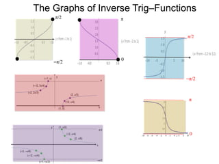
73. The Graphs of Inverse Trig–Functions

74. and the sine–inverse
y = sin–1(x) : [–1, 1] [–π/2, π/2].
We will use the variable x and y for the functions
y = sin(x): [–π/2, π/2] [–1, 1].
The Graphs of Inverse Trig–Functions

75. and the sine–inverse
y = sin–1(x) : [–1, 1] [–π/2, π/2].
We will use the variable x and y for the functions
y = sin(x): [–π/2, π/2] [–1, 1].
The Graphs of Inverse Trig–Functions
As in the case for all inverse pairs of functions,
the graph of y = sin–1(x) may be
obtained by reflecting
y = sin(x) across y = x.

76. –1
y = sin–1(x)
y = x
y = sin(x)
and the sine–inverse
y = sin–1(x) : [–1, 1] [–π/2, π/2].
We will use the variable x and y for the functions
y = sin(x): [–π/2, π/2] [–1, 1].
The Graphs of Inverse Trig–Functions
As in the case for all inverse pairs of functions,
the graph of y = sin–1(x) may be
obtained by reflecting
y = sin(x) across y = x.
–π/2 π/2
1
–1

77. –1
–π/2
y = sin–1(x)
1
–1
π/2
y = x
y = sin(x)
and the sine–inverse
y = sin–1(x) : [–1, 1] [–π/2, π/2].
We will use the variable x and y for the functions
y = sin(x): [–π/2, π/2] [–1, 1].
The Graphs of Inverse Trig–Functions
As in the case for all inverse pairs of functions,
the graph of y = sin–1(x) may be
obtained by reflecting
y = sin(x) across y = x.

78. –1
–π/2
1
–1
–π/2
π/2
1–1 π/2
y = x
y = sin(x)
and the sine–inverse
y = sin–1(x) : [–1, 1] [–π/2, π/2].
We will use the variable x and y for the functions
y = sin(x): [–π/2, π/2] [–1, 1].
The Graphs of Inverse Trig–Functions
As in the case for all inverse pairs of functions,
the graph of y = sin–1(x) may be
obtained by reflecting
y = sin(x) across y = x.
y = sin–1(x)

79. –1
–π/2
1
–1
–π/2
π/2
1–1 π/2
y = x
y = sin(x)
and the sine–inverse
y = sin–1(x) : [–1, 1] [–π/2, π/2].
We will use the variable x and y for the functions
y = sin(x): [–π/2, π/2] [–1, 1].
(π/6 ½)
The Graphs of Inverse Trig–Functions
As in the case for all inverse pairs of functions,
the graph of y = sin–1(x) may be
obtained by reflecting
y = sin(x) across y = x.
For example, the point
(π/6, ½) on y = sin(x)
y = sin–1(x)

80. –1
–π/2
1
–1
–π/2
π/2
1–1 π/2
y = x
y = sin(x)
and the sine–inverse
y = sin–1(x) : [–1, 1] [–π/2, π/2].
We will use the variable x and y for the functions
y = sin(x): [–π/2, π/2] [–1, 1].
(½, π/6)
(π/6 ½)
The Graphs of Inverse Trig–Functions
As in the case for all inverse pairs of functions,
the graph of y = sin–1(x) may be
obtained by reflecting
y = sin(x) across y = x.
For example, the point
(π/6, ½) on y = sin(x)
corresponds to (½, π/6)
on y = sin–1(x) since
(, a) and (a, ) are the
reflection of each other.
y = sin–1(x)

81. The graph of y = cos–1(x) is the reflection of the graph
of y = cos (x) where y = cos(x): [0, π] [–1, 1]
and y = cos–1(x): [–1, 1] [0, π]
The Graphs of Inverse Trig–Functions

82. The Graphs of Inverse Trig–Functions
y = x
π
0
1
–1
π
y = cos(x)
y = cos–1(x)
The graph of y = cos–1(x) is the reflection of the graph
of y = cos (x) where y = cos(x): [0, π] [–1, 1]
and y = cos–1(x): [–1, 1] [0, π]

83. The Graphs of Inverse Trig–Functions
y = x
π
0
1
–1
Here are some specific cosine inverse values:
π
(1, 0)
(–1, π)
(0, π/2)
cos–1(1) = 0,
cos–1(0) = π/2, and
cos–1(–1) = π.
y = cos(x)
y = cos–1(x)
The graph of y = cos–1(x) is the reflection of the graph
of y = cos (x) where y = cos(x): [0, π] [–1, 1]
and y = cos–1(x): [–1, 1] [0, π]

84. The Graphs of Inverse Trig–Functions
y = cos(x)
y = x
π
0
1
–1
Here are some specific cosine inverse values:
π
(1, 0)
(–1, π)
(0, π/2)
cos–1(1) = 0,
cos–1(0) = π/2, and
cos–1(–1) = π.
P  (0.74, 0.74) intersection point
P  (0.74, 0.74)
in radian.
By solving cos(x) = x
numerically, we've the
.y = cos–1(x)
The graph of y = cos–1(x) is the reflection of the graph
of y = cos (x) where y = cos(x): [0, π] [–1, 1]
and y = cos–1(x): [–1, 1] [0, π]

85. The domain of y = tan–1(x) is all real numbers and
the output y is restricted to –π/2 < y < π/2,
The Graphs of Inverse Trig–Functions

86. The domain of y = tan–1(x) is all real numbers and
the output y is restricted to –π/2 < y < π/2,
The Graphs of Inverse Trig–Functions
x
tan–1(x)
0 1/3 1 3 ∞–1/3–1–3–∞

87. The domain of y = tan–1(x) is all real numbers and
the output y is restricted to –π/2 < y < π/2,
The Graphs of Inverse Trig–Functions
x
tan–1(x)
0 1/3 1 3 ∞–1/3–1–3–∞
π/60 π/4 π/3 π/2

88. The domain of y = tan–1(x) is all real numbers and
the output y is restricted to –π/2 < y < π/2,
The Graphs of Inverse Trig–Functions
x
tan–1(x) π/60 π/4 π/3
0 1/3 1 3 ∞–1/3–1–3
π/2
–∞
y = π/2
(0,0)
(1,π/4)
(√3, π/3)

89. The domain of y = tan–1(x) is all real numbers and
the output y is restricted to –π/2 < y < π/2,
The Graphs of Inverse Trig–Functions
x
tan–1(x) π/60 π/4 π/3–π/2
0 1/3 1 3 ∞
–π/6
–1/3
–π/4
–1
–π/3
–3
π/2
–∞
y = π/2
(0,0)
(1,π/4)
(√3, π/3)

90. The domain of y = tan–1(x) is all real numbers and
the output y is restricted to –π/2 < y < π/2,
The Graphs of Inverse Trig–Functions
x
tan–1(x) π/60 π/4 π/3–π/2
0 1/3 1 3 ∞
–π/6
–1/3
–π/4
–1
–π/3
–3
π/2
–∞
y = π/2
y = –π/2
(0,0)
(1,π/4)
(–1,–π/4)
(√3, π/3)
(–√3, –π/3)

91. The domain of y = tan–1(x) is all real numbers and
the output y is restricted to –π/2 < y < π/2,
The Graphs of Inverse Trig–Functions
Here is the graph of y = tan–1(x)
x
tan–1(x) π/60 π/4 π/3–π/2
0 1/3 1 3 ∞
–π/6
–1/3
–π/4
–1
–π/3
–3
π/2
–∞
y = π/2
y = –π/2
(0,0)
(1,π/4)
(–1,–π/4)
(√3, π/3)
(–√3, –π/3)

92. The domain of y = tan–1(x) is all real numbers and
the output y is restricted to –π/2 < y < π/2,
The Graphs of Inverse Trig–Functions
Here is the graph of y = tan–1(x)
x
tan–1(x) π/60 π/4 π/3–π/2
0 1/3 1 3 ∞
–π/6
–1/3
–π/4
–1
–π/3
–3
π/2
–∞
y = π/2
y = –π/2
(0,0)
(1,π/4)
Remark: y =tan–1(x) has two horizontal asymptotes.
(–1,–π/4)
(√3, π/3)
(–√3, –π/3)

93. Inverse Trigonometric Functions
Cotangent–inverse is similar to tangent–inverse.
Given any number a, we define cot–1(a) = ,
where 0 <  < π and that cot() = a.
Cot–1(a) is also written as arccot(a) or acot(a).

94. Inverse Trigonometric Functions
Cotangent–inverse is similar to tangent–inverse.
Given any number a, we define cot–1(a) = ,
where 0 <  < π and that cot() = a.
Cot–1(a) is also written as arccot(a) or acot(a).
Here is the graph of y = cot–1(x)
(0, π/2)
(1, π/4)
x
y
π
(–1, 3π/4)
(√3, π/6)
(–√3, 5π/6)

95. The Graphs of Inverse Trig–Functions
For |a| ≥ 1, we define sec–1(a) =  with sec() = a,
where 0 <  < π,  ≠ π/2.
Sec–1(a) is also noted as arcsec(a) or asec(a).
Sin() and cos() vary between –1 and 1,
so their reciprocals |csc()| and |sec()| ≥ 1.

96. Using x and y, here is the graph of y = sec–1(x).
The Graphs of Inverse Trig–Functions
(1, 0) x
y
(√2, π/4)
(2, π/3)
(–1, π)
(–√2, 3π/4)
(–2, 2π/3)
For |a| ≥ 1, we define sec–1(a) =  with sec() = a,
where 0 <  < π,  ≠ π/2.
Sec–1(a) is also noted as arcsec(a) or asec(a).
Sin() and cos() vary between –1 and 1,
so their reciprocals |csc()| and |sec()| ≥ 1.
π

97. The Graphs of Inverse Trig–Functions
Given a number a such that |a| ≥ 1,
we define csc–1(a) =  with csc() = a
where –π/2 <  < π/2,  ≠ 0.
Csc–1(a) is also noted as arccsc (a) or acsc (a).

98. The Graphs of Inverse Trig–Functions
Given a number a such that |a| ≥ 1,
we define csc–1(a) =  with csc() = a
where –π/2 <  < π/2,  ≠ 0.
Csc–1(a) is also noted as arccsc (a) or acsc (a).
Using x and y, here is the graph of y = csc–1(x).
(1, π/2)
x
y
(–√2, –π/4)
(2, π/6)
(–1, –π/2)
(√2, π/4)
(–2, –π/6)
–π/2
π/2

99. –π/2
π/2
The Graphs of Inverse Trig–Functions
π
0
π/2
–π/2
π
0

100. One of the reasons for creating inverse functions is
for solving equations.
Linear Trig-Equations

101. One of the reasons for creating inverse functions is
for solving equations.
Linear Trig-Equations
The function 3x = y is different from x2 or sin(x)
in that if we know the output y = 1/2, then we know
the precise input x, in this case, 3x = ½, so x = 1/6.

102. One of the reasons for creating inverse functions is
for solving equations.
Linear Trig-Equations
Such is not the case for x2 or sin(x).
The function 3x = y is different from x2 or sin(x)
in that if we know the output y = 1/2, then we know
the precise input x, in this case, 3x = ½, so x = 1/6.

103. One of the reasons for creating inverse functions is
for solving equations.
Linear Trig-Equations
Such is not the case for x2 or sin(x).
If the output y = ½ so that x2 = ½ or sin(x) = ½,
we won’t be able to determine a precise input,
instead we have multiple or even infinite possibilities.
The function 3x = y is different from x2 or sin(x)
in that if we know the output y = 1/2, then we know
the precise input x, in this case, 3x = ½, so x = 1/6.

104. One of the reasons for creating inverse functions is
for solving equations.
Linear Trig-Equations
Such is not the case for x2 or sin(x).
If the output y = ½ so that x2 = ½ or sin(x) = ½,
we won’t be able to determine a precise input,
instead we have multiple or even infinite possibilities.
In these situations, we utilize trig-inverse functions to
obtain their solutions.
The function 3x = y is different from x2 or sin(x)
in that if we know the output y = 1/2, then we know
the precise input x, in this case, 3x = ½, so x = 1/6.

105. One of the reasons for creating inverse functions is
for solving equations.
Linear Trig-Equations
Such is not the case for x2 or sin(x).
If the output y = ½ so that x2 = ½ or sin(x) = ½,
we won’t be able to determine a precise input,
instead we have multiple or even infinite possibilities.
In these situations, we utilize trig-inverse functions to
obtain their solutions.
The function 3x = y is different from x2 or sin(x)
in that if we know the output y = 1/2, then we know
the precise input x, in this case, 3x = ½, so x = 1/6.
Specifically, we will solve linear trig-equations,
that is, equations of the form aX + b = 0
where X is a trig-function.

106. Important Trigonometric Values
Solving linear trig-equations is to solve for positions
on the unit circle.

107. Important Trigonometric Values
Solving linear trig-equations is to solve for positions
on the unit circle. From the position-solutions,
we apply the inverse trig-functions to obtain angular-
solutions and the list of all solutions, if necessary.

108. Important Trigonometric Values
Solving linear trig-equations is to solve for positions
on the unit circle. From the position-solutions,
we apply the inverse trig-functions to obtain angular-
solutions and the list of all solutions, if necessary.
Example g. a. Draw the two locations on the unit
circle corresponding to  where 5sin() – 3 = 0.

109. Important Trigonometric Values
Solving linear trig-equations is to solve for positions
on the unit circle. From the position-solutions,
we apply the inverse trig-functions to obtain angular-
solutions and the list of all solutions, if necessary.
Example g. a. Draw the two locations on the unit
circle corresponding to  where 5sin() – 3 = 0.
5sin() – 3 = 0 or
sin() = 3/5 = y-coordinate of the
point on the circle.

110. Important Trigonometric Values
Solving linear trig-equations is to solve for positions
on the unit circle. From the position-solutions,
we apply the inverse trig-functions to obtain angular-
solutions and the list of all solutions, if necessary.
Example g. a. Draw the two locations on the unit
circle corresponding to  where 5sin() – 3 = 0.
5sin() – 3 = 0 or
sin() = 3/5 = y-coordinate of the
point on the circle.
It’s positive so both points are at
the top-half of the circle as shown.
(–4/5, 3/5) (4/5, 3/5)

111. Important Trigonometric Values
Solving linear trig-equations is to solve for positions
on the unit circle. From the position-solutions,
we apply the inverse trig-functions to obtain angular-
solutions and the list of all solutions, if necessary.
By the Pythagorean Theorem we find
x = ±4/5 so the points are (4/5, 3/5) or (–4/5, 3/5).
Example g. a. Draw the two locations on the unit
circle corresponding to  where 5sin() – 3 = 0.
5sin() – 3 = 0 or
sin() = 3/5 = y-coordinate of the
point on the circle.
It’s positive so both points are at
the top-half of the circle as shown.
(–4/5, 3/5) (4/5, 3/5)

112. Important Trigonometric Values
b. Find the values of between 0 and π for the ’s.
(–4/5, 3/5) (4/5, 3/5)
A
Since sin() = 3/5, from the figure,
angle A is sin–1(3/5)  36.9o,

113. Important Trigonometric Values
b. Find the values of between 0 and π for the ’s.
Since sin() = 3/5, from the figure,
angle A is sin–1(3/5)  36.9o,
and angle B  180 – 36.9o = 143.1o
(–4/5, 3/5) (4/5, 3/5)
A
B

114. Important Trigonometric Values
b. Find the values of between 0 and π for the ’s.
Since sin() = 3/5, from the figure,
angle A is sin–1(3/5)  36.9o,
and angle B  180 – 36.9o = 143.1o
(–4/5, 3/5) (4/5, 3/5)
A
B
c. List all solutions of 5sin() – 3 = 0.

115. Important Trigonometric Values
b. Find the values of between 0 and π for the ’s.
Since sin() = 3/5, from the figure,
angle A is sin–1(3/5)  36.9o,
and angle B  180 – 36.9o = 143.1o
(–4/5, 3/5) (4/5, 3/5)
A
B
c. List all solutions of 5sin() – 3 = 0.
Each 360o corresponds to one cycle,
or that n360o corresponds to going around n times,
where n is an integer.

116. Important Trigonometric Values
b. Find the values of between 0 and π for the ’s.
Since sin() = 3/5, from the figure,
angle A is sin–1(3/5)  36.9o,
and angle B  180 – 36.9o = 143.1o
(–4/5, 3/5) (4/5, 3/5)
A
B
c. List all solutions of 5sin() – 3 = 0.
Each 360o corresponds to one cycle,
or that n360o corresponds to going around n times,
where n is an integer.
Hence the following is a complete list of solutions:
{36.9o+ n360o or 143.1o + n360o}

117. Important Trigonometric Values
b. Find the values of between 0 and π for the ’s.
Since sin() = 3/5, from the figure,
angle A is sin–1(3/5)  36.9o,
and angle B  180 – 36.9o = 143.1o
(–4/5, 3/5) (4/5, 3/5)
A
B
c. List all solutions of 5sin() – 3 = 0.
Each 360o corresponds to one cycle,
or that n360o corresponds to going around n times,
where n is an integer.
Hence the following is a complete list of solutions:
{36.9o+ n360o or 143.1o + n360o}
Sometimes we use the argument to π or 2π in the
equation to obtain answers in integers or fractions,
instead of answers in multiples of π.

118. Important Trigonometric Values
Example H.
a. Draw the two locations corresponding to angle α
on the unit circle where 2cos(α) – 1 = 0.

119. Important Trigonometric Values
Example H.
a. Draw the two locations corresponding to angle α
on the unit circle where 2cos(α) – 1 = 0.
We have 2cos(α) – 1 = 0
or cos(α) = ½ .

120. Important Trigonometric Values
Example H.
a. Draw the two locations corresponding to angle α
on the unit circle where 2cos(α) – 1 = 0. (1/2, √2/2)
(1/2, –√2/2)
We have 2cos(α) – 1 = 0
or cos(α) = ½ .
Hence the points are (1/2, √2/2)
and(1/2, –√2/2).

121. Important Trigonometric Values
Example H.
a. Draw the two locations corresponding to angle α
on the unit circle where 2cos(α) – 1 = 0.
b. List two angles for α that correspond
to the two points then list all the solutions for α.
We have 2cos(α) – 1 = 0
or cos(α) = ½ .
Hence the points are (1/2, √2/2)
and(1/2, –√2/2).
(1/2, √2/2)
(1/2, –√2/2)

122. Important Trigonometric Values
Example H.
a. Draw the two locations corresponding to angle α
on the unit circle where 2cos(α) – 1 = 0.
b. List two angles for α that correspond
to the two points then list all the solutions for α.
(1/2, √2/2)
(1/2, –√2/2)
We have 2cos(α) – 1 = 0
or cos(α) = ½ .
Hence the points are (1/2, √2/2)
and(1/2, –√2/2).
–π/3
π/3
Two angles for the positions are α = ±π/3.

123. Important Trigonometric Values
Example H.
a. Draw the two locations corresponding to angle α
on the unit circle where 2cos(α) – 1 = 0.
b. List two angles for α that correspond
to the two points then list all the solutions for α.
(1/2, √2/2)
(1/2, –√2/2)
We have 2cos(α) – 1 = 0
or cos(α) = ½ .
Hence the points are (1/2, √2/2)
and(1/2, –√2/2).
Two angles for the positions are α = ±π/3.
Hence a list for all the solutions for α is {±π/3 + 2nπ}.
–π/3
π/3

124. Important Trigonometric Values
Example H.
a. Draw the two locations corresponding to angle α
on the unit circle where 2cos(α) – 1 = 0.
b. List two angles for α that correspond
to the two points then list all the solutions for α.
(1/2, √2/2)
(1/2, –√2/2)
We have 2cos(α) – 1 = 0
or cos(α) = ½ .
Hence the points are (1/2, √2/2)
and(1/2, –√2/2).
Two angles for the positions are α = ±π/3.
Hence a list for all the solutions for α is {2nπ±π/3}.
c. Find all the solutions for  where 2cos(2π) – 1 = 0.
–π/3
π/3

125. Important Trigonometric Values
Example H.
a. Draw the two locations corresponding to angle α
on the unit circle where 2cos(α) – 1 = 0.
b. List two angles for α that correspond
to the two points then list all the solutions for α.
(1/2, √2/2)
(1/2, –√2/2)
We have 2cos(α) – 1 = 0
or cos(α) = ½ .
Hence the points are (1/2, √2/2)
and(1/2, –√2/2).
Two angles for the positions are α = ±π/3.
Hence a list for all the solutions for α is {2nπ±π/3}.
c. Find all the solutions for  where 2cos(2π) – 1 = 0.
We have that cos(2π) = ½ so 2π = 2nπ±π/3,
–π/3
π/3

126. Important Trigonometric Values
Example H.
a. Draw the two locations corresponding to angle α
on the unit circle where 2cos(α) – 1 = 0.
b. List two angles for α that correspond
to the two points then list all the solutions for α.
(1/2, √2/2)
A
B
(1/2, –√2/2)
We have 2cos(α) – 1 = 0
or cos(α) = ½ .
Hence the points are (1/2, √2/2)
and(1/2, –√2/2).
Two angles for the positions are α = ±π/3.
Hence a list for all the solutions for α is {2nπ±π/3}.
c. Find all the solutions for  where 2cos(2π) – 1 = 0.
We have that cos(2π) = ½ so 2π = 2nπ±π/3,
or  = (2nπ±π/3)/2π = n±1/6 where n is any integer.

127. Notes on Square–Sum Identities
Writing S(x) as S and replacing C2 as 1 – S2, we’ve
S2 – (1 – S2) = S or
2S2 – S – 1 = 0 so
(2S + 1)(S – 1) = 0
Hence 2S = 1, or S(x) = ½ so x = π/6 or 5π/6,
or that S = 1, so x = π/2.
Example I. Solve the equation
S2(x) – C2(x) = S(x).
a. Find all solutions x between 0 and 2π.
b. Find all solutions for x.
By adding 2nπ where n is an integer, to the solutions
from a. we obtain all the solutions for x. Here is a list:
{π/6 or π/2 or 5π/6 + 2nπ, where n is an integer}.

128. HW. A.
Linear Trig-Equations
Find the exact answers.
1. sin–1(0), sin–1(1), sin–1(–1), sin–1(1/2), sin–1(–1/2),
sin–1(√2/2), sin–1(–√2/2), sin–1(√3/2), sin–1(–√3/2),
2. List all the cosine inverses of the above values.
3. tan–1(0), tan–1(1), tan–1(–1), tan–1(√3), tan–1(–√3),
tan–1(1/√3), tan–1(–1/√3),
4. List all the cosine inverses of the values in 3.
5. Given A = sin–1(√3/2) find the exact values of
cos(A) and tan(A). Ans: ½, 1/√3
6. Given A = tan–1(3/2) find the exact values of
cos(A) and sin(A).

129. HW. A.
Linear Trig-Equations
7. Given A = cos–1(1/3) find the exact values of
sin (A) and tan(A).
8. Given A = tan–1(–4/3) find the exact values of
cos(A) and sin(A).
9. Find exact value of
sin–1(sin (π/3)), sin–1(sin(–π/3)), sin–1( sin(–4π/3)),
sin–1(sin(4π/3)),
10. Find exact value of
cos–1(sin(π/3)), cos–1( sin(–π/3)), cos–1( sin(–4π/3)),
cos–1(sin(4π/3)),

130. HW. B.
Linear Trig-Equations
1. Find the answer in terms of x
a. sin(cos–1(x)) b. cos(sin–1(x))
c. tan(sin–1(x)), d. sin(tan–1(x))
2. Find the answer in terms of x
a. sin(cos–1(x/2)) b. cos(sin–1(x/2))
c. tan(sin–1(x/2)), d. sin(tan–1(x/2))
3. Find the answer in terms of x
a. sin(cos–1(2/x)) b. cos(sin–1(2/x))
c. tan(sin–1(2/x)), d. sin(tan–1(2/x))

131. Linear Trig-Equations
Exercise. C.
Solve the following futons. equation S2(x) – C2(x) = S(x).
Find the x’s between 0 and 2π, then list all the solutions.
1. 2.
3. 4.
5. 6.
7. 8.
9. 10.
sin2 𝑥 − 1 = 0 4 cos2 𝑥 − 1 = 0
tan2 𝑥 − 3 = 0 cot2
𝑥 − 1 = 0
2sin2
𝑥 + sin (x) = 0 cos2 𝑥 − cos (x) = 0
tan 𝑥 = 1 cos 𝑥 = −
2
2
sin 𝑥 = −
1
2
sec 𝑥 = −2
9.
Ans:. 1.
𝜋
4
+ 𝑛𝜋 3.
7
6
𝜋 + 2𝑛𝜋,
11
6
𝜋 + 2𝑛𝜋
5.
𝜋
2
+ 𝑛𝜋 7.
𝜋
3
+ 2𝑛𝜋,
2𝜋
3
+ 2𝑛𝜋
𝑛𝜋,
7
6
𝜋 + 2𝑛𝜋,
11
6
𝜋 + 2𝑛𝜋