1. Deep Learning for Recommender Systems
Alexandros Karatzoglou (Scientific Director @ Telefonica Research)
alexk@tid.es, @alexk_z
Balázs Hidasi (Head of Research @ Gravity R&D)
balazs.hidasi@gravityrd.com, @balazshidasi
RecSys’17, 29 August 2017, Como

2. Why Deep Learning?
ImageNet challenge error rates (red line = human performance)

3. Why Deep Learning?

4. Complex Architectures

5. Neural Networks are Universal Function
Approximators

6. Inspiration for Neural Learning

7. Neural Model

8. Neuron a.k.a. Unit

9. Feedforward Multilayered Network

10. Learning

11. Stochastic Gradient Descent
• Generalization of (Stochastic) Gradient Descent

12. Stochastic Gradient Descent

13. Backpropagation

14. Backpropagation
• Does not work well in plain a
normal” multilayer deep network
• Vanishing Gradients
• Slow Learning
• SVM’s easier to train
• 2nd Neural Winter

15. Modern Deep Networks
• Ingredients:
• Rectified Linear Activation
function a.k.a. ReLu

16. Modern Deep Networks
• Ingredients:
• Dropout:

17. Modern Deep Networks
• Ingredients:
• Mini-batches:
– Stochastic Gradient Descent
– Compute gradient over many (50 -100) data points
(minibatch) and update.

18. Modern Feedforward Networks
• Ingredients:
• Adagrad a.k.a. adaptive learning rates

19. • Feature extraction directly from the content
• Image, text, audio, etc.
• Instead of metadata
• For hybrid algorithms
• Heterogenous data handled easily
• Dynamic/Sequential behaviour modeling with RNNs
• More accurate representation learning of users and items
• Natural extension of CF & more
• RecSys is a complex domain
• Deep learning worked well in other complex domains
• Worth a try
Deep Learning for RecSys

20. • As of 2017 summer, main topics:
• Learning item embeddings
• Deep collaborative filtering
• Feature extraction directly from content
• Session-based recommendations with RNN
• And their combinations
Research directions in DL-RecSys

21. • Start simple
• Add improvements later
• Optimize code
• GPU/CPU optimizations may differ
• Scalability is key
• Opensource code
• Experiment (also) on public datasets
• Don’t use very small datasets
• Don’t work on irrelevant tasks, e.g. rating prediction
Best practices

22. Item embeddings & 2vec models

23. Embeddings
• Embedding: a (learned) real value vector
representing an entity
– Also known as:
• Latent feature vector
• (Latent) representation
– Similar entities’ embeddings are similar
• Use in recommenders:
– Initialization of item representation in more advanced
algorithms
– Item-to-item recommendations

24. Matrix factorization as learning
embeddings
• MF: user & item embedding learning
– Similar feature vectors
• Two items are similar
• Two users are similar
• User prefers item
– MF representation as a simplictic neural
network
• Input: one-hot encoded user ID
• Input to hidden weights: user feature
matrix
• Hidden layer: user feature vector
• Hidden to output weights: item feature
matrix
• Output: preference (of the user) over the
items
R U
I
≈
0,0,...,0,1,0,0,...0
u
𝑟#,%, 𝑟#,&, … , 𝑟#,()
𝑊+
𝑊,

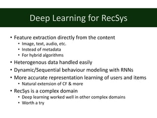
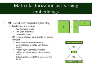
25. Word2Vec
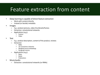
• [Mikolov et. al, 2013a]
• Representation learning of words
• Shallow model
• Data: (target) word + context pairs
– Sliding window on the document
– Context = words near the target
• In sliding window
• 1-5 words in both directions
• Two models
– Continous Bag of Words (CBOW)
– Skip-gram

26. Word2Vec - CBOW
• Continuous Bag of Words
• Maximalizes the probability of the target word given the
context
• Model
– Input: one-hot encoded words
– Input to hidden weights
• Embedding matrix of words
– Hidden layer
• Sum of the embeddings of the words in the context
– Hidden to output weights
– Softmax transformation
• Smooth approximation of the max operator
• Highlights the highest value
• 𝑠. =
012
∑ 0
145
467
, (𝑟8: scores)
– Output: likelihood of words of the corpus given the context
• Embeddings are taken from the input to hidden matrix
– Hidden to output matrix also has item representations (but not
used)
E E E E
𝑤:;& 𝑤:;% 𝑤:<% 𝑤:<&
word(t-2) word(t-1) word(t+2)word(t+1)
Classifier
averaging
0,1,0,0,1,0,0,1,0,1
𝑟. .=%
>
𝐸
𝑊
𝑝(𝑤.|𝑐) .=%
>
softmax
word(t)

27. Word2Vec – Skip-gram
• Maximalizes the probability of the
context, given the target word
• Model
– Input: one-hot encoded word
– Input to hidden matrix: embeddings
– Hidden state
• Item embedding of target
– Softmax transformation
– Output: likelihood of context words
(given the input word)
• Reported to be more accurate
E
𝑤:
word(t)
word(t-1) word(t+2)word(t+1)
Classifier
word(t-2)
0,0,0,0,1,0,0,0,0,0
𝑟. .=%
>
𝐸
𝑊
𝑝(𝑤.|𝑐) .=%
>
softmax

28. Geometry of the Embedding Space
King - Man + Woman = Queen

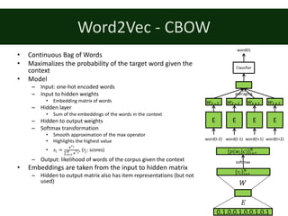
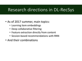
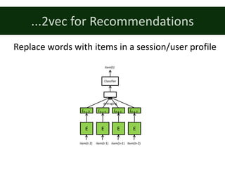
29. Paragraph2vec, doc2vec
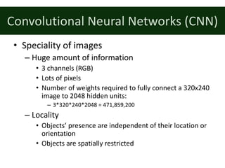
• [Le & Mikolov, 2014]
• Learns representation of
paragraph/document
• Based on CBOW model
• Paragraph/document
embedding added to the
model as global context
E E E E
𝑤:;& 𝑤:;% 𝑤:<% 𝑤:<&
word(t-2) word(t-1) word(t+2)word(t+1)
Classifier
word(t)
averaging
P
paragraph ID
𝑝.

30. ...2vec for Recommendations
Replace words with items in a session/user profile
E E E E
𝑖:;& 𝑖:;% 𝑖:<% 𝑖:<&
item(t-2) item(t-1) item(t+2)item(t+1)
Classifier
item(t)
averaging

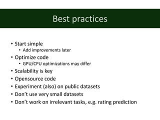
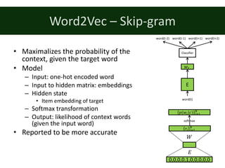
31. Prod2Vec
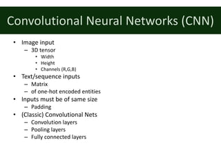
• [Grbovic et. al, 2015]
• Skip-gram model on products
– Input: i-th product purchased by the user
– Context: the other purchases of the user
• Bagged prod2vec model
– Input: products purchased in one basket by the user
• Basket: sum of product embeddings
– Context: other baskets of the user
• Learning user representation
– Follows paragraph2vec
– User embedding added as global context
– Input: user + products purchased except for the i-th
– Target: i-th product purchased by the user
• [Barkan & Koenigstein, 2016] proposed the same model later as item2vec
– Skip-gram with Negative Sampling (SGNS) is applied to event data

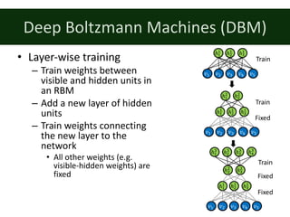
32. Prod2Vec
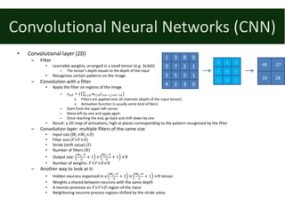
[Grbovic et. al, 2015]
pro2vec skip-gram model on products

33. Bagged Prod2Vec
[Grbovic et. al, 2015]
bagged-prod2vec model updates

34. User-Prod2Vec
[Grbovic et. al, 2015]
User embeddings for user to product predictions

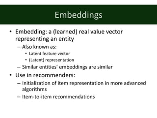
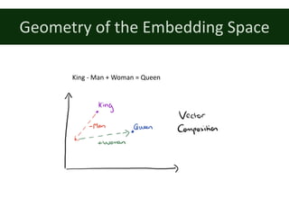
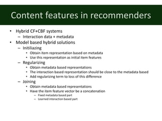
35. Utilizing more information
• Meta-Prod2vec [Vasile et. al, 2016]
– Based on the prod2vec model
– Uses item metadata
• Embedded metadata
• Added to both the input and the context
– Losses between: target/context item/metadata
• Final loss is the combination of 5 of these losses
• Content2vec [Nedelec et. al, 2017]
– Separate modules for multimodel information
• CF: Prod2vec
• Image: AlexNet (a type of CNN)
• Text: Word2Vec and TextCNN
– Learns pairwise similarities
• Likelihood of two items being bought together
I
𝑖:
item(t)
item(t-1) item(t+2)meta(t+1)
Classifier
meta(t-1)
M
𝑚:
meta(t)
Classifier Classifier Classifier Classifier
item(t)

36. References
• [Barkan & Koenigstein, 2016] O. Barkan, N. Koenigstein: ITEM2VEC: Neural item embedding for
collaborative filtering. IEEE 26th International Workshop on Machine Learning for Signal Processing
(MLSP 2016).
• [Grbovic et. al, 2015] M. Grbovic, V. Radosavljevic, N. Djuric, N. Bhamidipati, J. Savla, V. Bhagwan, D.
Sharp: E-commerce in Your Inbox: Product Recommendations at Scale. 21th ACM SIGKDD
International Conference on Knowledge Discovery and Data Mining (KDD’15).
• [Le & Mikolov, 2014] Q. Le, T. Mikolov: Distributed Representations of Sentences and Documents.
31st International Conference on Machine Learning (ICML 2014).
• [Mikolov et. al, 2013a] T. Mikolov, K. Chen, G. Corrado, J. Dean: Efficient Estimation of Word
Representations in Vector Space. ICLR 2013 Workshop.
• [Mikolov et. al, 2013b] T. Mikolov, I. Sutskever, K. Chen, G. Corrado, J. Dean: Distributed
Representations of Words and Phrases and Their Compositionality. 26th Advances in Neural
Information Processing Systems (NIPS 2013).
• [Morin & Bengio, 2005] F. Morin, Y. Bengio: Hierarchical probabilistic neural network language
model. International workshop on artificial intelligence and statistics, 2005.
• [Nedelec et. al, 2017] T. Nedelec, E. Smirnova, F. Vasile: Specializing Joint Representations for the
task of Product Recommendation. 2nd Workshop on Deep Learning for Recommendations (DLRS
2017).
• [Vasile et. al, 2016] F. Vasile, E. Smirnova, A. Conneau: Meta-Prod2Vec – Product Embeddings Using
Side-Information for Recommendations. 10th ACM Conference on Recommender Systems
(RecSys’16).

37. Deep Collaborative Filtering

38. CF with Neural Networks
• Natural application area
• Some exploration during the Netflix prize
• E.g.: NSVD1 [Paterek, 2007]
– Asymmetric MF
– The model:
• Input: sparse vector of interactions
– Item-NSVD1: ratings given for the item by users
» Alternatively: metadata of the item
– User-NSVD1: ratings given by the user
• Input to hidden weights: „secondary” feature vectors
• Hidden layer: item/user feature vector
• Hidden to output weights: user/item feature vectors
• Output:
– Item-NSVD1: predicted ratings on the item by all users
– User-NSVD1: predicted ratings of the user on all items
– Training with SGD
– Implicit counterpart by [Pilászy et. al, 2009]
– No non-linarities in the model
Ratings of the user
User features
Predicted ratings
Secondary feature
vectors
Item feature
vectors

39. Restricted Boltzmann Machines (RBM) for
recommendation
• RBM
– Generative stochastic neural network
– Visible & hidden units connected by (symmetric) weights
• Stochastic binary units
• Activation probabilities:
– 𝑝 ℎ8 = 1 𝑣 = 𝜎 𝑏8
L
+ ∑ 𝑤.,8 𝑣.
N
.=%
– 𝑝 𝑣. = 1 ℎ = 𝜎 𝑏.
O
+ ∑ 𝑤.,8ℎ8
P
8=%
– Training
• Set visible units based on data
• Sample hidden units
• Sample visible units
• Modify weights to approach the configuration of visible units to the data
• In recommenders [Salakhutdinov et. al, 2007]
– Visible units: ratings on the movie
• Softmax unit
– Vector of length 5 (for each rating value) in each unit
– Ratings are one-hot encoded
• Units correnponding to users who not rated the movie are ignored
– Hidden binary units
ℎQℎ&ℎ%
𝑣R𝑣S𝑣Q𝑣% 𝑣&
ℎQℎ&ℎ%
𝑣R𝑣S𝑣Q𝑣% 𝑣&
𝑟.: 2 ? ? 4 1

40. Deep Boltzmann Machines (DBM)
• Layer-wise training
– Train weights between
visible and hidden units in
an RBM
– Add a new layer of hidden
units
– Train weights connecting
the new layer to the
network
• All other weights (e.g.
visible-hidden weights) are
fixed
ℎQ
%
ℎ&
%
ℎ%
%
𝑣R𝑣S𝑣Q𝑣% 𝑣&
ℎQ
%
ℎ&
%
ℎ%
%
𝑣R𝑣S𝑣Q𝑣% 𝑣&
ℎ&
&
ℎ%
&
Train
Train
Fixed
ℎQ
%
ℎ&
%
ℎ%
%
𝑣R𝑣S𝑣Q𝑣% 𝑣&
ℎQ
&ℎ&
&
Train
Fixed
ℎ&
Qℎ%
Q ℎS
Q
ℎQ
Q
Fixed

41. Autoencoders
• Autoencoder
– One hidden layer
– Same number of input and output units
– Try to reconstruct the input on the output
– Hidden layer: compressed representation of the data
• Constraining the model: improve generalization
– Sparse autoencoders
• Activations of units are limited
• Activation penalty
• Requires the whole train set to compute
– Denoising autoencoders [Vincent et. al, 2008]
• Corrupt the input (e.g. set random values to zero)
• Restore the original on the output
• Deep version
– Stacked autoencoders
– Layerwise training (historically)
– End-to-end training (more recently)
Data
Corrupted input
Hidden layer
Reconstructed output
Data

42. Autoencoders for recommendation
• Reconstruct corrupted user interaction vectors
– CDL [Wang et. al, 2015]
Collaborative Deep Learning
Uses Bayesian stacked denoising autoencoders
Uses tags/metadata instead of the item ID

43. Autoencoders for recommendation
• Reconstruct corrupted user interaction vectors
– CDAE [Wu et. al, 2016]
Collaborative Denoising Auto-Encoder
Additional user node on the
input and bias node beside
the hidden layer

44. Recurrent autoencoder
• CRAE [Wang et. al, 2016]
– Collaborative Recurrent Autoencoder
– Encodes text (e.g. movie plot, review)
– Autoencoding with RNNs
• Encoder-decoder architecture
• The input is corrupted by replacing words with a
deisgnated BLANK token
– CDL model + text encoding simultaneously
• Joint learning

45. DeepCF methods
• MV-DNN [Elkahky et. al, 2015]
– Multi-domain recommender
– Separate feedforward networks for user and items per domain
(D+1 networks)
• Features first are embedded
• Run through several layers

46. DeepCF methods
• TDSSM [Song et. al, 2016]
• Temporal Deep Semantic Structured Model
• Similar to MV-DNN
• User features are the combination of a static and a temporal part
• The time dependent part is modeled by an RNN

47. DeepCF methods
• Coevolving features [Dai et. al, 2016]
• Users’ taste and items’ audiences change over time
• User/item features depend on time and are composed of
• Time drift vector
• Self evolution
• Co-evolution with items/users
• Interaction vector
Feature vectors are learned by RNNs

48. DeepCF methods
• Product Neural Network (PNN) [Qu et. al, 2016]
– For CTR estimation
– Embed features
– Pairwise layer: all pairwise combination
of embedded features
• Like Factorization Machines
• Outer/inner product of feature vectors or both
– Several fully connected layers
• CF-NADE [Zheng et. al, 2016]
– Neural Autoregressive Collaborative Filtering
– User events à preference (0/1) + confidence (based on occurence)
– Reconstructs some of the user events based on others (not the full set)
• Random ordering of user events
• Reconstruct the preference i, based on preferences and confidences up to i-1
– Loss is weighted by confidences

49. Applications: app recommendations
• Wide & Deep Learning [Cheng et. al, 2016]
• Ranking of results matching a query
• Combination of two models
– Deep neural network
• On embedded item features
• „Generalization”
– Linear model
• On embedded item features
• And cross product of item features
• „Memorization”
– Joint training
– Logistic loss
• Improved online performance
– +2.9% deep over wide
– +3.9% deep+wide over wide

50. Applications: video recommendations
• YouTube Recommender [Covington et. al, 2016]
– Two networks
– Candidate generation
• Recommendations as classification
– Items clicked / not clicked when were recommended
• Feedforward network on many features
– Average watch embedding vector of user (last few items)
– Average search embedding vector of user (last few searches)
– User attributes
– Geographic embedding
• Negative item sampling + softmax
– Reranking
• More features
– Actual video embedding
– Average video embedding of watched videos
– Language information
– Time since last watch
– Etc.
• Weighted logistic regression on the top of the network

51. References
• [Cheng et. al, 2016] HT. Cheng, L. Koc, J. Harmsen, T. Shaked, T. Chandra, H. Aradhye, G. Anderson, G. Corrado, W. Chai, M. Ispir, R.
Anil, Z. Haque, L. Hong, V. Jain, X. Liu, H. Shah: Wide & Deep Learning for Recommender Systems. 1st Workshop on Deep Learning for
Recommender Systems (DLRS 2016).
• [Covington et. al, 2016] P. Covington, J. Adams, E. Sargin: Deep Neural Networks for YouTube Recommendations. 10th ACM Conference
on Recommender Systems (RecSys’16).
• [Dai et. al, 2016] H. Dai, Y. Wang, R. Trivedi, L. Song: Recurrent Co-Evolutionary Latent Feature Processes for Continuous-time
Recommendation. 1st Workshop on Deep Learning for Recommender Systems (DLRS 2016).
• [Elkahky et. al, 2015] A. M. Elkahky, Y. Song, X. He: A Multi-View Deep Learning Approach for Cross Domain User Modeling in
Recommendation Systems. 24th International Conference on World Wide Web (WWW’15). [Paterek, 2007] A. Paterek: Improving
regularized singular value decomposition for collaborative filtering. KDD Cup and Workshop 2007.
• [Paterek, 2007] A. Paterek: Improving regularized singular value decomposition for collaborative filtering. KDD Cup 2007 Workshop.
• [Pilászy & Tikk, 2009] I. Pilászy, D. Tikk: Recommending new movies: even a few ratings are more valuable than metadata. 3rd ACM
Conference on Recommender Systems (RecSys’09).
• [Qu et. al, 2016] Y. Qu, H. Cai, K. Ren, W. Zhang, Y. Yu: Product-based Neural Networks for User Response Prediction. 16th International
Conference on Data Mining (ICDM 2016).
• [Salakhutdinov et. al, 2007] R. Salakhutdinov, A. Mnih, G. Hinton: Restricted Boltzmann Machines for Collaborative Filtering. 24th
International Conference on Machine Learning (ICML 2007).
• [Song et. al, 2016] Y. Song, A. M. Elkahky, X. He: Multi-Rate Deep Learning for Temporal Recommendation. 39th International ACM
SIGIR conference on Research and Development in Information Retrieval (SIGIR’16).
• [Vincent et. al, 2008] P. Vincent, H. Larochelle, Y. Bengio, P. A. Manzagol: Extracting and Composing Robust Features with Denoising
Autoencoders. 25th international Conference on Machine Learning (ICML 2008).
• [Wang et. al, 2015] H. Wang, N. Wang, DY. Yeung: Collaborative Deep Learning for Recommender Systems. 21th ACM SIGKDD
International Conference on Knowledge Discovery and Data Mining (KDD’15).
• [Wang et. al, 2016] H. Wang, X. Shi, DY. Yeung: Collaborative Recurrent Autoencoder: Recommend while Learning to Fill in the Blanks.
Advances in Neural Information Processing Systems (NIPS 2016).
• [Wu et. al, 2016] Y. Wu, C. DuBois, A. X. Zheng, M. Ester: Collaborative Denoising Auto-encoders for Top-n Recommender Systems. 9th
ACM International Conference on Web Search and Data Mining (WSDM’16)
• [Zheng et. al, 2016] Y. Zheng, C. Liu, B. Tang, H. Zhou: Neural Autoregressive Collaborative Filtering for Implicit Feedback. 1st Workshop
on Deep Learning for Recommender Systems (DLRS 2016).

52. Feature Extraction from Content

53. Content features in recommenders
• Hybrid CF+CBF systems
– Interaction data + metadata
• Model based hybrid solutions
– Initiliazing
• Obtain item representation based on metadata
• Use this representation as initial item features
– Regularizing
• Obtain metadata based representations
• The interaction based representation should be close to the metadata based
• Add regularizing term to loss of this difference
– Joining
• Obtain metadata based representations
• Have the item feature vector be a concatenation
– Fixed metadata based part
– Learned interaction based part

54. Feature extraction from content
• Deep learning is capable of direct feature extraction
– Work with content directly
– Instead (or beside) metadata
• Images
– E.g.: product pictures, video thumbnails/frames
– Extraction: convolutional networks
– Applications (e.g.):
• Fashion
• Video
• Text
– E.g.: product description, content of the product, reviews
– Extraction
• RNNs
• 1D convolution networks
• Weighted word embeddings
• Paragraph vectors
– Applications (e.g.):
• News
• Books
• Publications
• Music/audio
– Extraction: convolutional networks (or RNNs)

55. Convolutional Neural Networks (CNN)
• Speciality of images
– Huge amount of information
• 3 channels (RGB)
• Lots of pixels
• Number of weights required to fully connect a 320x240
image to 2048 hidden units:
– 3*320*240*2048 = 471,859,200
– Locality
• Objects’ presence are independent of their location or
orientation
• Objects are spatially restricted

56. Convolutional Neural Networks (CNN)
• Image input
– 3D tensor
• Width
• Height
• Channels (R,G,B)
• Text/sequence inputs
– Matrix
– of one-hot encoded entities
• Inputs must be of same size
– Padding
• (Classic) Convolutional Nets
– Convolution layers
– Pooling layers
– Fully connected layers

57. Convolutional Neural Networks (CNN)
• Convolutional layer (2D)
– Filter
• Learnable weights, arranged in a small tensor (e.g. 3x3xD)
– The tensor’s depth equals to the depth of the input
• Recognizes certain patterns on the image
– Convolution with a filter
• Apply the filter on regions of the image
– 𝑦V,W = 𝑓 ∑ 𝑤.,8,Y 𝐼.<V;%,8<W;%,Y.,8,Y
» Filters are applied over all channels (depth of the input tensor)
» Activation function is usually some kind of ReLU
– Start from the upper left corner
– Move left by one and apply again
– Once reaching the end, go back and shift down by one
• Result: a 2D map of activations, high at places corresponding to the pattern recognized by the filter
– Convolution layer: multiple filters of the same size
• Input size (𝑊%×𝑊&×𝐷)
• Filter size (𝐹×𝐹×𝐷)
• Stride (shift value) (𝑆)
• Number of filters (𝑁)
• Output size:
a7;b
(
+ 1 ×
ac;b
(
+ 1 ×𝑁
• Number of weights: 𝐹×𝐹×𝐷×𝑁
– Another way to look at it:
• Hidden neurons organized in a
a7;b
(
+ 1 ×
ac;b
(
+ 1 ×𝑁 tensor
• Weights a shared between neurons with the same depth
• A neuron processe an 𝐹×𝐹×𝐷 region of the input
• Neighboring neurons process regions shifted by the stride value
1 3 8 0
0 7 2 1
2 5 5 1
4 2 3 0
-1 -2 -1
-2 12 -2
-1 -2 -1
48 -27
19 28

58. Convolutional Neural Networks (CNN)
• Pooling layer
– Mean pooling: replace an 𝑅×𝑅 region with the mean of the values
– Max pooling: replace an 𝑅×𝑅 region with the maximum of the values
– Used to quickly reduce the size
– Cheap, but very aggressive operator
• Avoid when possible
• Often needed, because convolutions don’t decrease the number of inputs fast enough
– Input size: 𝑊%×𝑊&×𝑁
– Output size:
a7
e
×
ac
e
×𝑁
• Fully connected layers
– Final few layers
– Each hidden neuron is connected with every neuron in the next layer
• Residual connections (improvement) [He et. al, 2016]
– Very deep networks degrade performance
– Hard to find the proper mappings
– Reformulation of the problem: F(x) à F(x)+x
Layer
Layer
+
𝑥
𝐹 𝑥 + 𝑥
𝐹(𝑥)

59. Convolutional Neural Networks (CNN)
• Some examples
• GoogLeNet [Szegedy et. al, 2015]
• Inception-v3 model [Szegedy et. al, 2016]
• ResNet (up to 200+ layers) [He et. al, 2016]

60. Images in recommenders
• [McAuley et. Al, 2015]
– Learns a parameterized distance metric over visual
features
• Visual features are extracted from a pretrained CNN
• Distance function: Eucledian distance of „embedded” visual
features
– Embedding here: multiplication with a weight matrix to reduce
the number of dimensions
– Personalized distance
• Reweights the distance with a user specific weight vector
– Training: maximizing likelihood of an existing
relationship with the target item
• Over uniformly sampled negative items

61. Images in recommenders
• Visual BPR [He & McAuley, 2016]
– Model composed of
• Bias terms
• MF model
• Visual part
– Pretrained CNN features
– Dimension reduction through „embedding”
– The product of this visual item feature and a learned user feature vector is used in the
model
• Visual bias
– Product of the pretrained CNN features and a global bias vector over its features
– BPR loss
– Tested on clothing datasets (9-25% improvement)

62. Music representations
• [Oord et. al, 2013]
– Extends iALS/WMF with audio
features
• To overcome cold-start
– Music feature extraction
• Time-frequency representation
• Applied CNN on 3 second
samples
• Latent factor of the clip: average
predictions on consecutive
windows of the clip
– Integration with MF
• (a) Minimize distance between
music features and the MF’s
feature vectors
• (b) Replace the item features
with the music features
(minimize original loss)

63. Textual information improving
recommendations
• [Bansal et. al, 2016]
– Paper recommendation
– Item representation
• Text representation
– Two layer GRU (RNN): bidirectional layer followed by a unidirectional layer
– Representation is created by pooling over the hidden states of the sequence
• ID based representation (item feature vector)
• Final representation: ID + text added
– Multi-task learning
• Predict both user scores
• And likelihood of tags
– End-to-end training
• All parameters are trained simultaneously (no pretraining)
• Loss
– User scores: weighted MSE (like in iALS)
– Tags: weighted log likelihood (unobserved tags are downweighted)

64. References
• [Bansal et. al, 2016] T. Bansal, D. Belanger, A. McCallum: Ask the GRU: Multi-Task
Learning for Deep Text Recommendations. 10th ACM Conference on
Recommender Systems (RecSys’16).
• [He et. al, 2016] K. He, X. Zhang, S. Ren, J. Sun: Deep Residual Learning for Image
Recognition. CVPR 2016.
• [He & McAuley, 2016] R. He, J. McAuley: VBPR: Visual Bayesian Personalized
Ranking from Implicit Feedback. 30th AAAI Conference on Artificial Intelligence
(AAAI’ 16).
• [McAuley et. Al, 2015] J. McAuley, C. Targett, Q. Shi, A. Hengel: Image-based
Recommendations on Styles and Substitutes. 38th International ACM SIGIR
Conference on Research and Development in Information Retrieval (SIGIR’15).
• [Oord et. al, 2013] A. Oord, S. Dieleman, B. Schrauwen: Deep Content-based Music
Recommendation. Advances in Neural Information Processing Systems (NIPS
2013).
• [Szegedy et. al, 2015] C. Szegedy, W. Liu, Y. Jia, P. Sermanet, S. Reed, D. Anguelov,
D. Erhan, V. Vanhoucke, A. Rabinovich: Going Deeper with Convolutions. CVPR
2015.
• [Szegedy et. al, 2016] C. Szegedy, V. Vanhoucke, S. Ioffe, J. Shlens, Z. Wojna:
Rethinking the Inception Architecture for Computer Vision. CVPR 2016.

65. Session-based Recommendations with
RNNs

66. Recurrent Neural Networks
• Input: sequential information ( 𝑥: :=%
g
)
• Hidden state (ℎ:):
– representation of the sequence so far
– influenced by every element of the sequence up
to t
• ℎ: = 𝑓 𝑊𝑥: + 𝑈ℎ:;% + 𝑏

67. RNN-based machine learning
• Sequence to value
– Encoding, labeling
– E.g.: time series classification
• Value to sequence
– Decoding, generation
– E.g.: sequence generation
• Sequence to sequence
– Simultaneous
• E.g.: next-click prediction
– Encoder-decoder architecture
• E.g.: machine translation
• Two RNNs (encoder & decoder)
– Encoder produces a vector describing the sequence
» Last hidden state
» Combination of hidden states (e.g. mean pooling)
» Learned combination of hidden states
– Decoder receives the summary and generates a new sequence
» The generated symbol is usually fed back to the decoder
» The summary vector can be used to initialize the decoder
» Or can be given as a global context
• Attention mechanism (optionally)
ℎ% ℎ& ℎQ
𝑥% 𝑥& 𝑥Q
𝑦
ℎ% ℎ& ℎQ
𝑥
𝑦% 𝑦& 𝑦Q
ℎ% ℎ& ℎQ
𝑥% 𝑥& 𝑥Q
𝑦% 𝑦& 𝑦Q
ℎ%
0
ℎ&
0
ℎQ
0
𝑥% 𝑥& 𝑥Q
𝑦% 𝑦& 𝑦Q
ℎ%
i
ℎ&
i
ℎQ
i
𝑠
𝑠 𝑠 𝑠𝑦% 𝑦&0

68. Exploding/Vanishing gradients
• ℎ: = 𝑓 𝑊𝑥: + 𝑈ℎ:;% + 𝑏
• Gradient of ℎ: wrt. 𝑥%
– Simplification: linear activations
• In reality: bounded
–
kLl
km7
=
kLl
kLln7
kLln7
kLlnc
⋯
kLc
kL7
kL7
km7
= 𝑈:;%
𝑊
• 𝑈 & < 1 à vanishing gradients
– The effect of values further in the past is neglected
– The network forgets
• 𝑈 & > 1 à exploding gradients
– Gradients become very large on longer sequences
– The network becomes unstable

69. Handling exploding gradients
• Gradient clipping
– If the gradient is larger than a threshold, scale it back to
the threshold
– Updates are not accurate
– Vanishing gradients are not solved
• Enforce 𝑈 & = 1
– Unitary RNN
– Unable to forget
• Gated networks
– Long-Short Term Memory (LSTM)
– Gated Recurrent Unit (GRU)
– (and a some other variants)

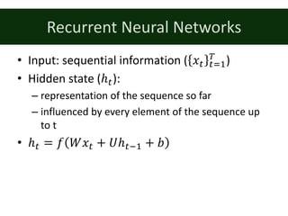
70. Long-Short Term Memory (LSTM)
• [Hochreiter & Schmidhuber, 1999]
• Instead of rewriting the hidden state during update,
add a delta
– 𝑠: = 𝑠:;% + Δ𝑠:
– Keeps the contribution of earlier inputs relevant
• Information flow is controlled by gates
– Gates depend on input and the hidden state
– Between 0 and 1
– Forget gate (f): 0/1 à reset/keep hidden state
– Input gate (i): 0/1 à don’t/do consider the contribution of
the input
– Output gate (o): how much of the memory is written to the
hidden state
• Hidden state is separated into two (read before you
write)
– Memory cell (c): internal state of the LSTM cell
– Hidden state (h): influences gates, updated from the
memory cell
𝑓: = 𝜎 𝑊s 𝑥: + 𝑈sℎ:;% + 𝑏s
𝑖: = 𝜎 𝑊. 𝑥: + 𝑈.ℎ:;% + 𝑏.
𝑜: = 𝜎 𝑊u 𝑥: + 𝑈uℎ:;% + 𝑏u
𝑐̃: = tanh 𝑊𝑥: + 𝑈ℎ:;% + 𝑏
𝑐: = 𝑓: ∘ 𝑐:;% + 𝑖: ∘ 𝑐̃:
ℎ: = 𝑜: ∘ tanh 𝑐:
𝐶
ℎ
IN
OUT
+
+
i
f
o

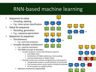
71. Gated Recurrent Unit (GRU)
• [Cho et. al, 2014]
• Simplified information flow
– Single hidden state
– Input and forget gate merged à
update gate (z)
– No output gate
– Reset gate (r) to break
information flow from previous
hidden state
• Similar performance to LSTM ℎ
r
IN
OUT
z
+
𝑧: = 𝜎 𝑊~ 𝑥: + 𝑈~ℎ:;% + 𝑏~
𝑟: = 𝜎 𝑊• 𝑥: + 𝑈•ℎ:;% + 𝑏•
ℎ€: = tanh 𝑊𝑥: + 𝑟: ∘ 𝑈ℎ:;% + 𝑏
ℎ: = 𝑧: ∘ ℎ: + 1 − 𝑧: ∘ ℎ€:

72. Session-based recommendations
• Sequence of events
– User identification problem
– Disjoint sessions (instead of consistent user history)
• Tasks
– Next click prediction
– Predicting intent
• Classic algorithms can’t cope with it well
– Item-to-item recommendations as approximation in
live systems
• Area revitalized by RNNs

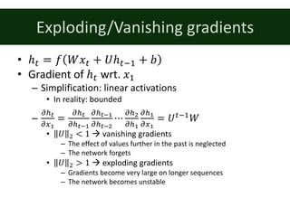
73. GRU4Rec (1/3)
• [Hidasi et. al, 2015]
• Network structure
– Input: one hot encoded item ID
– Optional embedding layer
– GRU layer(s)
– Output: scores over all items
– Target: the next item in the session
• Adapting GRU to session-based
recommendations
– Sessions of (very) different length & lots of short
sessions: session-parallel mini-batching
– Lots of items (inputs, outputs): sampling on the
output
– The goal is ranking: listwise loss functions on
pointwise/pairwise scores
GRU layer
One-hot vector
Weighted output
Scores on items
f()
One-hot vector
ItemID (next)
ItemID

74. GRU4Rec (2/3)
• Session-parallel mini-batches
– Mini-batch is defined over sessions
– Update with one step BPTT
• Lots of sessions are very short
• 2D mini-batching, updating on longer
sequences (with or without padding) didn’t
improve accuracy
• Output sampling
– Computing scores for all items (100K – 1M) in
every step is slow
– One positive item (target) + several samples
– Fast solution: scores on mini-batch targets
• Items of the other mini-batch are negative
samples for the current mini-batch
• Loss functions
– Cross-entropy + softmax
– Average of BPR scores
– TOP1 score (average of ranking error +
regularization over score values)
𝑖%,% 𝑖%,& 𝑖%,Q 𝑖%,S
𝑖&,% 𝑖&,& 𝑖&,Q
𝑖Q,% 𝑖Q,& 𝑖Q,Q 𝑖Q,S 𝑖Q,R 𝑖Q,‚
𝑖S,% 𝑖S,&
𝑖R,% 𝑖R,& 𝑖R,Q
Session1
Session2
Session3
Session4
Session5
𝑖%,% 𝑖%,& 𝑖%,Q
𝑖&,% 𝑖&,&
𝑖Q,% 𝑖Q,& 𝑖Q,Q 𝑖Q,S 𝑖Q,R
𝑖S,%
𝑖R,% 𝑖R,&
Input
Desired
output
…
𝑖%,& 𝑖%,Q 𝑖%,S
𝑖&,& 𝑖&,Q
𝑖Q,& 𝑖Q,Q 𝑖Q,S 𝑖Q,R 𝑖Q,‚
𝑖S,&
𝑖R,& 𝑖R,Q
…
𝑖% 𝑖R 𝑖ƒ
𝑦„%
%
𝑦„&
%
𝑦„Q
% 𝑦„S
%
𝑦„R
%
𝑦„‚
% 𝑦„…
%
𝑦„ƒ
%
𝑦„%
Q
𝑦„&
Q
𝑦„Q
Q
𝑦„S
Q
𝑦„R
Q
𝑦„‚
Q
𝑦„…
Q
𝑦„ƒ
Q
𝑦„%
&
𝑦„&
&
𝑦„Q
& 𝑦„S
&
𝑦„R
&
𝑦„‚
& 𝑦„…
&
𝑦„ƒ
&
1 0 0 0 0 0 0 0
0 0 0 0 0 0 0 1
0 0 0 0 1 0 0 0
𝑋𝐸 = − log 𝑠. , 𝑠. =
0Š‹2
∑ 0
Š‹45Œ
467
𝐵𝑃𝑅 =
− ∑ log 𝜎 𝑦„. − 𝑦„8
>Œ
8=%
𝑁(
𝑇𝑂𝑃1 =
∑ 𝜎 𝑦„8 − 𝑦„.
>Œ
8=% + ∑ 𝜎 𝑦„8
&>Œ
8=%
𝑁(

75. GRU4Rec (3/3)
• Observations
– Similar accuracy with/without embedding
– Multiple layers rarely help
• Sometimes slight improvement with 2 layers
• Sessions span over short time, no need for multiple time scales
– Quick conversion: only small changes after 5-10 epochs
– Upper bound for model capacity
• No improvement when adding additional units after a certain
threshold
• This threshold can be lowered with some techniques
• Results
– 20-30% improvement over item-to-item recommendations

76. Improving GRU4Rec
• Recall@20 on RSC15 by GRU4Rec: 0.6069 (100 units), 0.6322 (1000 units)
• Data augmentation [Tan et. al, 2016]
– Generate additional sessions by taking every possible sequence starting from the end of a session
– Randomly remove items from these sequences
– Long training times
– Recall@20 on RSC15 (using the full training set for training): ~0.685 (100 units)
• Bayesian version (ReLeVar) [Chatzis et. al, 2017]
– Bayesian formulation of the model
– Basically additional regularization by adding random noise during sampling
– Recall@20 on RSC15: 0.6507 (1500 units)
• New losses and additional sampling [Hidasi & Karatzoglou, 2017]
– Use additional samples beside minibatch samples
– Design better loss functions
• BPR”•– = − log ∑ 𝑠8 𝜎 𝑟. − 𝑟8
>Œ
8=% + 𝜆 ∑ 𝑟8
&>Œ
8=%
– Recall@20 on RSC15: 0.7119 (100 units)

77. Extensions
• Multi-modal information (p-RNN model) [Hidasi et. al, 2016]
– Use image and description besides the item ID
– One RNN per information source
– Hidden states concatenated
– Alternating training
• Item metadata [Twardowski, 2016]
– Embed item metadata
– Merge with the hidden layer of the RNN (session representation)
– Predict compatibility using feedforward layers
• Contextualization [Smirnova & Vasile, 2017]
– Merging both current and next context
– Current context on the input module
– Next context on the output module
– The RNN cell is redefined to learn context-aware transitions
• Personalizing by inter-session modeling
– Hierarchical RNNs [Quadrana et. al, 2017], [Ruocco et. al, 2017]
• One RNN works within the session (next click prediction)
• The other RNN predicts the transition between the sessions of the user

78. References
• [Chatzis et. al, 2017] S. P. Chatzis, P. Christodoulou, A. Andreou: Recurrent Latent Variable Networks for Session-Based
Recommendation. 2nd Workshop on Deep Learning for Recommender Systems (DLRS 2017).
https://arxiv.org/abs/1706.04026
• [Cho et. al, 2014] K. Cho, B. van Merrienboer, D. Bahdanau, Y. Bengio. On the properties of neural machine translation:
Encoder-decoder approaches. https://arxiv.org/abs/1409.1259
• [Hidasi et. al, 2015] B. Hidasi, A. Karatzoglou, L. Baltrunas, D. Tikk: Session-based Recommendations with Recurrent Neural
Networks. International Conference on Learning Representations (ICLR 2016). https://arxiv.org/abs/1511.06939
• [Hidasi et. al, 2016] B. Hidasi, M. Quadrana, A. Karatzoglou, D. Tikk: Parallel Recurrent Neural Network Architectures for
Feature-rich Session-based Recommendations. 10th ACM Conference on Recommender Systems (RecSys’16).
• [Hidasi & Karatzoglou, 2017] B. Hidasi, Alexandros Karatzoglou: Recurrent Neural Networks with Top-k Gains for Session-
based Recommendations. https://arxiv.org/abs/1706.03847
• [Hochreiter & Schmidhuber, 1997] S. Hochreiter, J. Schmidhuber: Long Short-term Memory. Neural Computation, 9(8):1735-
1780.
• [Quadrana et. al, 2017]:M. Quadrana, A. Karatzoglou, B. Hidasi, P. Cremonesi: Personalizing Session-based
Recommendations with Hierarchical Recurrent Neural Networks. 11th ACM Conference on Recommender Systems
(RecSys’17). https://arxiv.org/abs/1706.04148
• [Ruocco et. al, 2017]: M. Ruocco, O. S. Lillestøl Skrede, H. Langseth: Inter-Session Modeling for Session-Based
Recommendation. 2nd Workshop on Deep Learning for Recommendations (DLRS 2017). https://arxiv.org/abs/1706.07506
• [Smirnova & Vasile, 2017] E. Smirnova, F. Vasile: Contextual Sequence Modeling for Recommendation with Recurrent Neural
Networks. 2nd Workshop on Deep Learning for Recommender Systems (DLRS 2017). https://arxiv.org/abs/1706.07684
• [Tan et. al, 2016] Y. K. Tan, X. Xu, Y. Liu: Improved Recurrent Neural Networks for Session-based Recommendations. 1st
Workshop on Deep Learning for Recommendations (DLRS 2016). https://arxiv.org/abs/1606.08117
• [Twardowski, 2016] B. Twardowski: Modelling Contextual Information in Session-Aware Recommender Systems with Neural
Networks. 10th ACM Conference on Recommender Systems (RecSys’16).

79. Conclusions
• Deep Learning is now in RecSys
• Huge potential, but lot to do
– E.g. Explore more advanced DL techniques
• Current research directions
– Item embeddings
– Deep collaborative filtering
– Feature extraction from content
– Session-based recommendations with RNNs
• Scalability should be kept in mind
• Don’t fall for the hype BUT don’t disregard the
achievements of DL and its potential for RecSys

80. Thank you!