This document provides instructions for manually equalizing the histograms of two X-ray computed tomography (XCT) subvolumes measured under similar conditions using ImageJ software. The key steps are: 1. Open both subvolumes in ImageJ and identify overlapping slices between them. 2. Duplicate the overlapping slices and obtain histograms to adjust brightness/contrast values iteratively until the histograms are equalized. 3. Convert both subvolumes to 8-bit, apply the brightness/contrast values to equalize the histograms, and concatenate the subvolumes into a single volume.

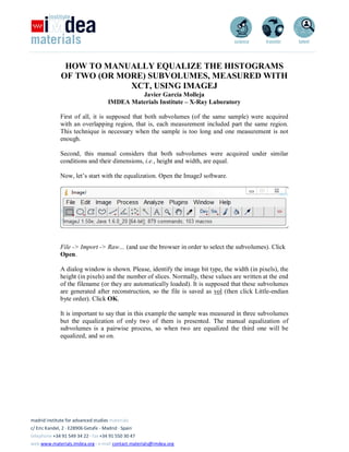
1. madrid institute for advanced studies materials
c/ Eric Kandel, 2 · E28906 Getafe - Madrid · Spain
telephone +34 91 549 34 22 · fax +34 91 550 30 47
web www.materials.imdea.org · e-mail contact.materials@imdea.org
HOW TO MANUALLY EQUALIZE THE HISTOGRAMS
OF TWO (OR MORE) SUBVOLUMES, MEASURED WITH
XCT, USING IMAGEJ
Javier García Molleja
IMDEA Materials Institute – X-Ray Laboratory
First of all, it is supposed that both subvolumes (of the same sample) were acquired
with an overlapping region, that is, each measurement included part the same region.
This technique is necessary when the sample is too long and one measurement is not
enough.
Second, this manual considers that both subvolumes were acquired under similar
conditions and their dimensions, i.e., height and width, are equal.
Now, let’s start with the equalization. Open the ImageJ software.
File -> Import -> Raw… (and use the browser in order to select the subvolumes). Click
Open.
A dialog window is shown. Please, identify the image bit type, the width (in pixels), the
height (in pixels) and the number of slices. Normally, these values are written at the end
of the filename (or they are automatically loaded). It is supposed that these subvolumes
are generated after reconstruction, so the file is saved as vol (then click Little-endian
byte order). Click OK.
It is important to say that in this example the sample was measured in three subvolumes
but the equalization of only two of them is presented. The manual equalization of
subvolumes is a pairwise process, so when two are equalized the third one will be
equalized, and so on.

2. 2
The volume is loaded in the TOP-BOTTOM view. Now, it is time to identify which
subvolume represents the top part of the sample and which one represents the middle
part of the sample.
TOP REGION MIDDLE REGION
Next step is to locate a slice, without artifacts, repeated in both subvolumes. If the
overlapped region is in the upper side of the sample, the identical slice must be at the
end of the top subvolume and at the beginning of the middle subvolume. Please, write
the number of slice in both cases.
Of course, the overlapped region will contain many slices. The choice of two identical
slices depends on you (or if one volume is better than the other and you want to
minimize the bad one…)

3. 3
TOP SLICE #1916 MIDDLE SLICE #432
Image -> Duplicate… these identical slices. Please, give them different names in order
to know which is which and do not check Duplicate stack option.
In the present case, there is a xls file named (ask me if you want to do by yourself)
XX_Gray_level_equalization_YY_(REF_ZZ)_v02.xls
XX means the number of file used in the complete volume (01 in the present case; the
equalization of the concatenated top-middle volume with the bottom subvolume will be
02); YY is the subvolume to be histogram-equalized and ZZ is the subvolume of
reference. In this moment, you can select one of these slices as reference, i.e., the one
with the “true” histogram. In this case, randomly, top subvolume is the one to be
equalized and the middle subvolume has the “real” histogram.
Image -> Type -> 8-bit the slice of the subvolume of reference (the middle one in this
example).
Analyze -> Histogram in order to obtain the histogram of this slice.

4. 4
Click List in order to obtain the histogram in a numerical representation.
In this window go to Edit -> Select All and then Edit -> Copy and go to the xls file and
then to the REF_middle_MAT+BKG_8b tab. Paste the values at the ‘bin start’ and
‘count’ columns.
Now, adjust the X and Y ranges of the three plots, namely, BKG (stands for the peak of
the histogram identified as the gray values of the background), MAT (stands for the
peak of the histogram identified as the gray values of the material) and ALL (stands for
the complete histogram).
To adjust the plots you may need to check:
https://excel.tips.net/T003031_Changing_the_Axis_Scale.html

5. 5
There are two boxes with black borders: one for the background and another for the
material. Please, give for RANGE BKG and for RANGE MAT extreme gray values (X1
is the minimum one and X2 is the maximum one), far away for each peak. Normally,
they can be selected similar to the X and Y ranges of the plots. On the other hand, for
THR BKG and THR MAT you should select the threshold of the peak, that is, from
zero counts to the selected value all gray values will be considered not belonging to the
peak. These values will be dependent on the user expertise, so please, feel free to
change or adjust to the most suitable for you and for the present subvolumes!
This process will be repeated with the slice to be equalized. Start with the histogram,
open the list, select the data and copy them in the up_MAT+BKG_16b tab in the Excel
file (in the ‘bin start’ and ‘count’ columns).

6. 6
Now, you need to do the same than before: adjust the X and Y ranges of the three plots,
write proper values for RANGE BKG X1, X2 and for RANGE MAT X1 and X2 and fill
the values corresponding to THR BKG and THR MAT. Hey! Bear in mind the decimal
separator is ‘.’ in ImageJ.
If you go to the Hoja1 tab you will see the column named ‘Iteracion’. Both, x and y
values are in blue color.
Image -> Duplicate… the slice from the top subvolume.
Image -> Adjust -> Brightness/Contrast…

7. 7
Click the Set button and put ‘Iteracion x’ as Minimum displayed value and ‘Iteracion y’
as Maximum displayed value. Select Automatic in Unsigned 16-bit range and do not
check Propagate to all other open images. In the present case the blue numbers are 3492
and 40124. Click OK.
Image -> Type -> 8-bit to this duplicated slice.
Analyze -> Histogram and click List button in order to select all columns and copy
them to up_MAT+BKG_8b tab in the Excel file (in the ‘bin start’ and ‘count’
columns). Now, repeat the same than before (adjust the ranges of all the plots, insert
proper values for RANGE BKG -X1 and X2-, RANGE MAT -X1 and X2- and select
THR BKG and THR MAT values).

8. 8
In the gray cells near to the ones with the black border there are a couple of numbers,
namely, INT BKG and INT MAT. Please, write these values (129.19 and 226.57 in the
present case) in Hoja1 tab, in MEDIA A’ and in MEDIA B’ rows (they are in gray
color, near to the blue values).
Pay attention to the ‘correction’ row, if its absolute value is lesser than 1 both slices are
equalized by their histograms. If its absolute value is greater than 1, a second iteration
will be needed. In the present case, correction is -1.26006, so both slices are not well
equalized.

9. 9
The row number 5 is automatically filled and you need to copy the new blue values, i.e.,
‘Iteracion x’ and ‘Iteracion y’ values.
Go to the slice from the top subvolume (the one of 16-bit).
Image -> Duplicate… for a second time.
Image -> Adjust -> Brightness/Contrast… and click the Set button in order to put these
new couple of minimum and maximum displayed values. In the present case, these new
numbers are, respectively, 3673 and 40305. Click OK.
Image -> Type -> 8-bit. After this, the process is repeated: obtain the histogram, click
the List button, select all data and copy them to the up_MAT+BKG_8b tab in the ‘bin
start’ and ‘count’ columns. See the change in the gray cells.
Write INT BKG and INT MAT in Hoja1 tab in MEDIA A’ and MEDIA B’ columns (in
the row number 5).
In the present case ‘correction’ has a value of 0.09 so the histograms are equalized and a
third iteration is not necessary. However, if you are too obsesive try to repeat the
process until ‘correction’ value tends to 0. Furthermore, you need to copy and paste this
row number 5 in the number 6 in order to continue the process!
I know, this is a repetitive and confusing task but it is a very confident process! Now it
is time to equalize both subvolumes. Remember that we were working with slices so
far. First of all, go to the reference subvolume (the middle one in this example).
Image -> Type -> 8-bit.

10. 10
Go to the other subvolume, that is, the top one.
Image -> Adjust -> Brightness/Contrast… and click the Set button. Use the two last
blue values (remember, 3673 and 40305) in order to set the minimum and maximum
displayed values and click OK.
Image -> Type -> 8-bit in order to match the bit type of both equalized subvolumes.
TOP BOTTOM
Now it is time to concatenate both subvolumes! Sorry, but these next steps are detailed
in another manual. Get it!
After concatenation, you can adjust the brightness and the contrast in order to optimize
them and do a rescale (the minumum gray value will be zero and the maximum gray
value will be 255).

11. 11
Image -> Adjust -> Brightness/Contrast… and go to a slice with neither shadows nor
artifacts, click Auto button and then the Apply button. And save the concatenated
volume! Furthermore, save the Excel file!
(Thanks to Juan Ignacio Caballero for the the critical reading of this manual and several
useful tips.)