
Recommended
Recommended
More Related Content
Similar to ENGR 102B Microsoft Excel Proficiency LevelsPlease have your in.docx
Similar to ENGR 102B Microsoft Excel Proficiency LevelsPlease have your in.docx (20)
More from YASHU40
More from YASHU40 (20)
Recently uploaded
Recently uploaded (20)
ENGR 102B Microsoft Excel Proficiency LevelsPlease have your in.docx
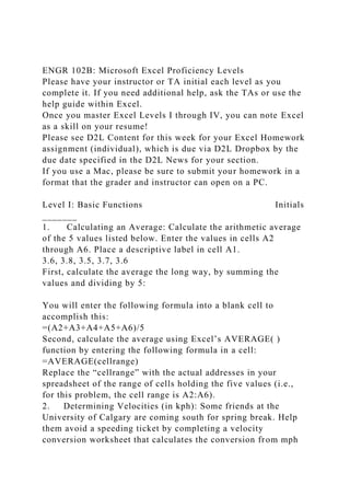
- 1. ENGR 102B: Microsoft Excel Proficiency Levels Please have your instructor or TA initial each level as you complete it. If you need additional help, ask the TAs or use the help guide within Excel. Once you master Excel Levels I through IV, you can note Excel as a skill on your resume! Please see D2L Content for this week for your Excel Homework assignment (individual), which is due via D2L Dropbox by the due date specified in the D2L News for your section. If you use a Mac, please be sure to submit your homework in a format that the grader and instructor can open on a PC. Level I: Basic Functions Initials _______ 1. Calculating an Average: Calculate the arithmetic average of the 5 values listed below. Enter the values in cells A2 through A6. Place a descriptive label in cell A1. 3.6, 3.8, 3.5, 3.7, 3.6 First, calculate the average the long way, by summing the values and dividing by 5: You will enter the following formula into a blank cell to accomplish this: =(A2+A3+A4+A5+A6)/5 Second, calculate the average using Excel’s AVERAGE( ) function by entering the following formula in a cell: =AVERAGE(cellrange) Replace the “cellrange” with the actual addresses in your spreadsheet of the range of cells holding the five values (i.e., for this problem, the cell range is A2:A6). 2. Determining Velocities (in kph): Some friends at the University of Calgary are coming south for spring break. Help them avoid a speeding ticket by completing a velocity conversion worksheet that calculates the conversion from mph
- 2. to kph in increments of 10 from 10 to 100. A conversion factor you will need is 0.62 miles/km; you will need this factor to convert from miles/hour to km/hour. Place the conversion factor in its own cell and then reference it in your conversion calculations using absolute cell referencing (e.g., $C$2). Refer to the CBT video on Absolute and Relative Cell Referencing from the “Preparation for the Excel Workshop” assignment if you don’t remember how to do this. Level II: Advanced Functions Initials _______ 1. Projectile Motion I: (See following page for Fig. 1 Excel chart) A projectile is launched at the angle 35o from the horizontal with a velocity equal to 30 m/s. Neglecting air resistance and assuming a horizontal surface, determine how far away from the launch site the projectile will land. To answer this problem, you will need: 1. Excel’s trigonometry functions to handle the 35o angle, and 2. Equations relating distance to velocity and acceleration When velocity is constant, as in the horizontal motion of our particle (since we’re neglecting air resistance), the distance traveled is simply the initial horizontal velocity times the time of flight: (Equation 1) What keeps the projectile from flying forever is gravity. Since the gravitational acceleration is constant, the vertical distance traveled becomes (Equation 2) Because the projectile ends up back on the ground, the final value of y is zero (a horizontal surface was specified), so Equation 2 can be used to determine the time of flight, t: t = 2(voy)/g, where g = 9.8 m/s2 (Equation 3) The initial velocity components in the horizontal and vertical directions can be determined with Excel’s trigonometry functions, as shown in Figure 1 (following page).
- 3. In Figure 1, Cells C6 and C7 must contain the following formulas: Cell C6: =C4*SIN(RADIANS(C3)) Cell C7: =C4*COS(RADIANS(C3)) The RADIANS( ) function has been used to convert 35o to radians for compatibility with Excel’s trigonometric functions. Once your spreadsheet has calculated V0y and V0x, you can use Equation 3 to solve for the time of flight in Figure 1. The time of flight can then be used in Equation 1 to find the horizontal distance traveled. A B C D 1 PROJECTILE MOTION 1 2 3 Angle: 35 degrees 4 V0:
- 5. m/s2 12 t: * s 13 14 HORIZONTAL TRAVEL DISTANCE 15 16 x: * m * = insert appropriate formula (Figure 1) Checking your answers: Given the information above, your spreadsheet should calculate
- 6. that for V0 = 30 m/s and the launch angle = 35 degrees, V0y = 17.21 m/s and V0x = 24.57 m/s. In addition, your spreadsheet should calculate that t = 3.51 s and x = 86.30 m. If your spreadsheet is not giving you these results, your formulas are likely incorrect, so keep working. 2. Projectile Motion II: How do the flight time and horizontal distance traveled change if the launch angle is decreased to 30 degrees (launch speed is unchanged)? Level III: Using Excel for Statistics Initials _______ 1. Statistics: Sixty transducers are tested to see how long they work without failure in a given environment. Rather than typing in the data, use Excel’s random number generator to generate 60 data points between 0 and 3 (one way to do this is to type “=RAND()*3”). You may notice that the sixty randomly-generated values change each time you make changes to other areas of your worksheet. You should “freeze” these values by copying them and then using “Paste Options: Values” to paste the random number values into an adjacent column. Use Excel’s statistical functions—AVERAGE, MEDIAN, MAX, MIN, STDEV.S, and QUARTILE.INC—to calculate statistics for your “frozen” data (calculate the 1st, 2nd, and 3rd quartiles; check to see whether your calculated 2nd Quartile = median). 2. Statistics, continued: For the data you generated in (1.) above, generate a histogram, which is a type of graph that shows the relative frequency of occurrences: Decrease the number of decimal places for your data to two. Use the “Number” tab on Excel’s ribbon to accomplish this. Determine a suitable X-axis range for the histogram. In general,
- 7. you could find the range for your X-axis by subtracting the MIN value from the MAX value. In this particular case, you know your data ranges from 0 to 3, so use this as your range. Determine the number of “bins” – recall that a good rule of thumb is that the number of bins should roughly equal the square root of n. What is the value of n in this case? Now take the square root of n and round it to the nearest odd number. Divide the range by the number of bins to determine the size of each bin. Since you now know the range and the number and size of the bins, you can set up a table from which your histogram can be constructed. Your table will have two columns: ‘Bin” and “Number of Occurrences.” The value in the “Bin” column will be equal to the high value of each bin range. Populate this table using an analysis of your sixty values. You may want to sort your sixty random numbers from low to high in order to make this step easier (Editing => Sort & Filter). Now use Excel to construct your histogram chart. One way to do this is to highlight your table’s number of occurrences data and go to Insert => Column => 2-D Column. Then use the bin data to adjust your X-axis values. To accomplish this, first click on the X-axis values to highlight them, then go to Chart Tools => Design => Select Data. Click on “Edit” under Horizontal (Category) Axis Labels, then fill in the range where your bin values are located under the “Add Label Range” field. Now click “OK.” Click “OK” again in the Select Data Source window. The Y-axis values should already depict the frequency of occurrence for each of the bins. Be sure to remove the space between the columns to create a proper histogram. To do this, select the data series in the plot: right-click on one of the columns, then => Format Data Series => Series Options => Gap Width => 0%. Label the axes appropriately and title your graph. Level IV: Using Excel for Graphing and Charts Initials _______ 1. Graphing: Use the Temperature and Time data below. Enter the data, then:
- 8. A B C 1 Temperature vs. Time Data 2 3 Time (Sec) Temp (C) 4 0 54.23 5 1 45.75 6 2 28.41 7 3 28.3 8 4 26.45
- 10. 18 14 0.32 19 15 1.68 (A) Create a scatter plot of the data (Insert/Charts/Scatter). Label the axes and give your graph a title (click on chart; Chart Tools/Design/Chart Layouts/Quick Layout). (B) Add a trendline and display R2 (a measure of the “goodness of fit”) (Chart Tools/Layout/Analysis/Trendline). To add a trendline, you can also right click on the data points and go to “Add trendline.” See if you can choose a type of trendline that gives you an R2 very close to 1.0, which means that your trendline formula is a good fit for your data points. 2. Advanced Graphing: The surface plot in Figure 2 shows the value of F(X,Y) = sin(X) * cos(Y) for -1 X 2 and -1 Y 2. You will be reproducing this surface plot. (Figure 2) (A) Create the table for F(X,Y) = sin (X) cos (Y) for the ranges -1 ≤ X ≤ 2 and -1 ≤ Y ≤ 2. Remember to use the $ sign where appropriate in your formulas for absolute cell addressing. To create the table, X values ranging from -1 to 2 should be entered in column A with increments of .2, and Y values ranging from -1 to 2 should be entered in row 2, also with increments of .2. The first two values are entered by hand, and then Excel’s Fill Handle (small square that appears in the bottom right corner of the selected cells) can be used to complete the rest of each series. See Figure 3 for illustration of the first part of the chart (note: the whole chart is not displayed
- 11. below – you will need to create it within your spreadsheet). … . (Figure 3) . . (B) Graph the resulting surface area data (Insert/Charts/Other Charts => Surface => “Wire frame” icon). (C) Label the axes appropriately and title your graph. ***************************************************** ********** F(X,Y) = sin (X) cos (Y) -1 -1 -0.8 -0.6 -0.4 -0.2 0 0.2 0.4 0.6 0.8 1 1.2 1.4 1.6 1.8 2 -0.45464871341284091 - 0.58625848083662813 -0.6944959726750779 - 0.77504610169174781 -0.8246975884333746 - 0.8414709848078965 -0.8246975884333746 - 0.77504610169174781 -0.6944959726750779 - 0.58625848083662813 -0.45464871341284091 - 0.30491353651226449 -0.1430224191212503 2.4570550786785637E-2 0.19118397037180895 0.35017548837401463 -0.8 -1 -0.8 -0.6 -0.4 -0.2 0 0.2 0.4 0.6 0.8 1 1.2 1.4 1.6 1.8 2 - 0.38758915004156702 -0.49978680152075255 - 0.59205953039176074 -0.66072871413793843 - 0.70305672910146599 -0.71735609089952279 - 0.70305672910146599 -0.66072871413793843 - 0.59205953039176074 -0.49978680152075255 - 0.38758915004156702 -0.25993954225851562 - 0.12192696521227749 2.0946455174185981E-2 0.16298480649321617 0.29852546790566076 -0.6 -1 -0.8 -0.6 -0.4 -0.2 0 0.2 0.4 0.6 0.8 1 1.2 1.4 1.6 1.8 2 -0.30507763036642738 - 0.39339019959669946 -0.4660195429836132 - 0.52007015780147892 -0.55338721660408663 - 0.56464247339503537 -0.55338721660408663 -
- 12. 0.52007015780147892 -0.4660195429836132 - 0.39339019959669946 -0.30507763036642738 - 0.20460257874157994 -9.5970667963079528E-2 1.6487290494153213E-2 0.12828795270803775 0.23497417908349799 -0.4 -1 -0.8 -0.6 -0.4 -0.2 0 0.2 0.4 0.6 0.8 1 1.2 1.4 1.6 1.8 2 - 0.21040362829671244 -0.27131037182928791 - 0.3214008270064177 -0.3586780454497614 - 0.38165590209504829 -0.38941834230865052 - 0.38165590209504829 -0.3586780454497614 - 0.3214008270064177 -0.27131037182928791 - 0.21040362829671244 -0.14110875607099124 - 6.6188323035149377E-2 1.1370829570772362E-2 8.8476663084435025E-2 0.16205521124517713 -0.2 -1 -0.8 -0.6 -0.4 -0.2 0 0.2 0.4 0.6 0.8 1 1.2 1.4 1.6 1.8 2 -0.1073414975338518 - 0.13841425570643057 -0.16396887429543613 - 0.18298657129998708 -0.19470917115432523 - 0.19866933079506122 -0.19470917115432523 - 0.18298657129998708 -0.16396887429543613 - 0.13841425570643057 -0.1073414975338518 - 7.1989372590281847E-2 -3.3767258537139425E-2 5.8010495551325146E-3 4.5138088107911742E-2 8.26756135293025E-2 0 -1 -0.8 -0.6 -0.4 -0.2 0 0.2 0.4 0.6 0.8 1 1.2 1.4 1.6 1.8 2 0 0 0 0 0 0 0 0 0 0 0 0 0 0 0 0 0.2 -1 -0.8 -0.6 -0.4 -0.2 0 0.2 0.4 0.6 0.8 1 1.2 1.4 1.6 1.8 2 0.1073414975338518 0.13841425570643057 0.16396887429543613 0.18298657129998708 0.19470917115432523 0.19866933079506122 0.19470917115432523 0.18298657129998708 0.16396887429543613 0.13841425570643057 0.1073414975338518 7.1989372590281847E-2 3.3767258537139425E-2 -5.8010495551325146E-3- 4.5138088107911742E-2 -8.26756135293025E-2 0.4 -1 -
- 13. 0.8 -0.6 -0.4 -0.2 0 0.2 0.4 0.6 0.8 1 1.2 1.4 1.6 1.8 2 0.21040362829671244 0.27131037182928791 0.3214008270064177 0.3586780454497614 0.38165590209504829 0.38941834230865052 0.38165590209504829 0.3586780454497614 0.3214008270064177 0.27131037182928791 0.21040362829671244 0.14110875607099124 6.6188323035149377E-2 - 1.1370829570772362E-2 -8.8476663084435025E-2- 0.16205521124517713 0.6 -1 -0.8 -0.6 -0.4 -0.2 0 0.2 0.4 0.6 0.8 1 1.2 1.4 1.6 1.8 2 0.30507763036642738 0.39339019959669946 0.4660195429836132 0.52007015780147892 0.55338721660408663 0.56464247339503537 0.55338721660408663 0.52007015780147892 0.4660195429836132 0.39339019959669946 0.30507763036642738 0.20460257874157994 9.5970667963079528E-2 -1.6487290494153213E-2- 0.12828795270803775 -0.23497417908349799 0.8 -1 - 0.8 -0.6 -0.4 -0.2 0 0.2 0.4 0.6 0.8 1 1.2 1.4 1.6 1.8 2 0.38758915004156702 0.49978680152075255 0.59205953039176074 0.66072871413793843 0.70305672910146599 0.71735609089952279 0.70305672910146599 0.66072871413793843 0.59205953039176074 0.49978680152075255 0.38758915004156702 0.25993954225851562 0.12192696521227749 - 2.0946455174185981E-2 -0.16298480649321617 - 0.29852546790566076 1 -1 -0.8 -0.6 -0.4 -0.2 0 0.2 0.4 0.6 0.8 1 1.2 1.4 1.6 1.8 2 0.45464871341284091 0.58625848083662813 0.6944959726750779 0.77504610169174781 0.8246975884333746 0.8414709848078965 0.8246975884333746 0.77504610169174781 0.6944959726750779 0.58625848083662813 0.45464871341284091 0.30491353651226449
- 14. 0.1430224191212503 -2.4570550786785637E-2- 0.19118397037180895 -0.35017548837401463 1.2 -1 - 0.8 -0.6 -0.4 -0.2 0 0.2 0.4 0.6 0.8 1 1.2 1.4 1.6 1.8 2 0.50358286730732571 0.64935788456716603 0.7692450521366152 0.85846484697051395 0.91346035739817832 0.93203908596722629 0.91346035739817832 0.85846484697051395 0.7692450521366152 0.64935788456716603 0.50358286730732571 0.33773159027557548 0.15841602051320158 - 2.7215096076372867E-2 -0.21176123266758409 - 0.38786511716355132 1.4 -1 -0.8 -0.6 -0.4 -0.2 0 0.2 0.4 0.6 0.8 1 1.2 1.4 1.6 1.8 2 0.53244076142990071 0.68656943860731268 0.81332675886260219 0.90765930784304583 0.96580634450436575 0.98544972998846014 0.96580634450436575 0.90765930784304583 0.81332675886260219 0.68656943860731268 0.53244076142990071 0.35708535130826274 0.16749407507795255 -2.8774661367597085E-2- 0.22389624286811524 -0.41009178771093335 1.6 -1 - 0.8 -0.6 -0.4 -0.2 0 0.2 0.4 0.6 0.8 1 1.2 1.4 1.6 1.8 2 0.54007192260824977 0.69640963572533676 0.8249836943137433 0.920668256396454 0.97964868043332765 0.99957360304150511 0.97964868043332765 0.920668256396454 0.8249836943137433 0.69640963572533676 0.54007192260824977 0.36220324623227773 0.16989466942746431 - 2.9187071713790043E-2 -0.2271052164109463 - 0.41596939280175144 1.8 -1 -0.8 -0.6 -0.4 -0.2 0 0.2 0.4 0.6 0.8 1 1.2 1.4 1.6 1.8 2 0.52617212052771389 0.67848617831468028 0.80375113325918868 0.89697306690402512 0.95443551493359335 0.97384763087819515 0.95443551493359335 0.89697306690402512
- 15. 0.80375113325918868 0.67848617831468028 0.52617212052771389 0.35288124072745131 0.16552209944053539 -2.8435885615885139E-2- 0.22126022164742623 -0.40526361086889012 2 -1 - 0.8 -0.6 -0.4 -0.2 0 0.2 0.4 0.6 0.8 1 1.2 1.4 1.6 1.8 2 0.49129549643388193 0.63351361806156559 0.75047555090496221 0.83751839179632803 0.89117201734889273 0.90929742682568171 0.89117201734889273 0.83751839179632803 0.75047555090496221 0.63351361806156559 0.49129549643388193 0.32949097373597147 0.1545506856841021 - 2.6551050493101028E-2 -0.20659428007382899 - 0.37840124765396416 X F(X,Y) Y [1] X↓Y→ -1-0.8-0.6-0.4-0.200.20.40.60.811.2 -1-0.45-0.59-0.69-0.78-0.82-0.84-0.82-0.78-0.69-0.59-0.45-0.30 -0.8-0.39-0.50-0.59-0.66-0.70-0.72-0.70-0.66-0.59-0.50-0.39- 0.26 -0.6-0.31-0.39-0.47-0.52-0.55-0.56-0.55-0.52-0.47-0.39-0.31- 0.20 -0.4-0.21-0.27-0.32-0.36-0.38-0.39-0.38-0.36-0.32-0.27-0.21- 0.14 -0.2-0.11-0.14-0.16-0.18-0.19-0.20-0.19-0.18-0.16-0.14-0.11- 0.07 00.000.000.000.000.000.000.000.000.000.000.000.00 0.20.110.140.160.180.190.200.190.180.160.140.110.07 0.40.210.270.320.360.380.390.380.360.320.270.210.14