czczz

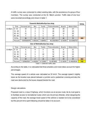
1. A traffic survey was conducted to collect existing data, with the assistance of a group of four
members. The survey was conducted at the St. Mary's junction. Traffic data of one hour
were recorded accordingly and shown in table 1.
Towards Mattakkuliya bus stop TOTAL
Time Personal cars Bus Trucks Three wheelers Bicycle Motor bikes
15.40pm 0 - 15 12 3 3 58 20 17
15 - 30 8 3 5 49 10 10
30 - 45 11 5 5 51 13 20
45 - 60 7 2 1 19 5 23
TOTAL 38 13 14 177 48 70 360
Percent 9.947643979 3.403141 3.664921 46.33507853 12.56545 18.32460733
Out of Mattakkuliya bus stop
Time Personal cars Bus Trucks Three wheelers Bicycle Motor bikes
15.40pm 0 - 15 6 4 4 61 9 11
15 - 30 5 3 1 55 13 13
30 - 45 11 5 10 52 10 24
45 - 60 6 5 3 44 16 11
TOTAL 28 17 18 212 48 59 382
Percent 7.329842932 4.450262 4.712042 55.4973822 12.56545 15.44502618 742
Table 1. Collected traffic data
According to the table, it is noticeable that three wheelers and motor bikes account for higher
percentages.
The average speed of a vehicle was calculated as 22 km/h. The average speed it slightly
lower as the location was placed between a junction and a pedestrian crossing and also the
road was destructed by the buses stopped beside the road.
Design calculations
Proposed road is a class II highway, which functions as an access route. As its main goal is
to facilitate access to recreational routes which are not primary Arterials, when designing the
capacity of the road, the average travel speed of the vehicle is needed not to be considered
but the percent time spent following should be taken in to account.

2. The following table 2 shows the level of service criteria for two lane highways in class II.
Level of service Percent time spent following Average travel speed km/h
A ≤ 35 >90
B >35 – 50 > 80-90
G >50-65 > 70-80
D >65-80 > 60-70
E >80 ≤ 60
Table 2. Level of service criteria for two-lane highways in class II (Exhibit 20-2)
The capacity design of the proposed road sectionfor present condition is as follows:
Percent time spent following Mean speed
V 15,max = 105 + 112 = 217
V 15,max = maximum volume within 15 minutes
V = 742 veh/hour
V = Demand volume for the full peak hour
𝑽 𝒑 =
𝑽
𝑷𝑯𝑭 ∗ 𝑭 𝑮 ∗ 𝒇 𝑯𝑽
(20-3)[4]
 𝐕 𝐩 = 𝐩𝐚𝐬𝐬𝐞𝐧𝐠𝐞𝐫 𝐜𝐚𝐫 𝐞𝐪𝐮𝐢𝐯𝐚𝐥𝐞𝐧𝐭 𝐟𝐥𝐨𝐰 𝐟𝐨𝐫 𝟏𝟓 𝐦𝐢𝐧 𝐩𝐞𝐫𝐢𝐨𝐝 𝐩𝐜/𝐡)
𝑷𝑯𝑭 =
𝑽
𝑽 𝟏𝟓 ∗ 𝟒
=
𝟕𝟒𝟐
𝟐𝟏𝟕∗𝟒
= 0.855
 PHF = peak hour factor
𝒇 𝑯𝑽 =
𝟏
𝟏+𝑷 𝑻 (𝑬 𝑻−𝟏)+𝑷 𝑹 (𝑬 𝑹−𝟏)
(20-4)[4]
 f HV = heavy vehicle factor
ET = 1.1
ER = 0
FG = 1(Terrain = level)
ET = 1.2
ER = 0
FG = 1(Terrain = level)

3. (Exhibit 20-10)[4] (Exhibit 20-9)[4]
PT =
𝟔𝟐
𝟕𝟒𝟐
∗ 𝟏𝟎𝟎%= 8.4% = 0.084 (considering buses and trucks)
𝒇
𝑯𝑽 =
𝟏
𝟏+𝟎.𝟎𝟖𝟒( 𝟏.𝟏−𝟏)+𝟎
= 0.992
𝑓
𝐻𝑉 =
1
1+0.084(1.2−1)+0
= 0.983
VP =
𝟕𝟒𝟐
𝟎.𝟖𝟓𝟓∗𝟏∗𝟎.𝟗𝟗𝟐
= 875 VP =
742
0.855∗1∗0.983
= 883
 Lane width = 6.6m
 Drain width = 0.45m
 Shoulder width = 0m
FLS = 6.8 (Exhibit 20-5)[4]
Considering 14 access points,
fA= (12-8/6)*2 + 8 = 9.33 kmh-1
(Exhibit 20-6)[4]
BFFS = 110 kmh-1
(for urban areas)
FFS = BFFS – FLS -fA(20-2)[4]
= 110 – 6.8 – 9.33 = 93.87 kmh-1
PTSF = BPTSF +fd/np(20-12)[4]
BPTSF = 100 (1 - e-0.000879Vp) (20-7)
= 100 (1 - e-0.000879 * 875) = 53.66 kmh-1
ATS = FFS – 0.0125Vp - fnp(20-5)[4]
fnp = 0 (T.20-11)
ATS = 93.87 – 0.0125*883 – 0 = 82.84 kmh-1
Level Of service = C

4. Present Level of service = C
The capacity design of the proposed road section in 20 years condition is as follows:
 The growth rate of vehicles in 20 years is considered as 4%
Percent time spent following Mean speed
V = 1596
V 15,max = 421
𝑽 𝒑 =
𝑽
𝑷𝑯𝑭∗𝑭 𝑮∗𝒇 𝑯𝑽
(20-3) [4]
𝑷𝑯𝑭 =
𝑽
𝑽 𝟏𝟓 ∗ 𝟒
=
𝟏𝟓𝟗𝟔
𝟒𝟐𝟏∗𝟒
= 0.948
𝒇 𝑯𝑽 =
𝟏
𝟏+𝑷 𝑻 (𝑬 𝑻−𝟏)+𝑷 𝑹 (𝑬 𝑹−𝟏)
(20-4) [4]
ET = 1.0
ER = 0
FG = 1(Terrain = level) (Exhibit 20-10) [4]
ET = 1.1
ER = 0
FG = 1(Terrain = level)(Exhibit 20-9)[4]
PT =
𝟗𝟏
𝟏𝟓𝟗𝟔
∗ 𝟏𝟎𝟎%= 5.7% = 0.057 (considering buses and trucks)
𝒇
𝑯𝑽 =
𝟏
𝟏+𝟎.𝟎𝟓𝟕( 𝟏.𝟎−𝟏)+𝟎
= 1
𝑓
𝐻𝑉 =
1
1+0.057(1.1−1)+0
= 0.994
VP =
𝟏𝟓𝟗𝟔
𝟎.𝟗𝟒𝟖∗𝟏∗𝟏
= 1684 VP =
1596
0.948∗1∗1
= 1694

5.  Lane width = 6.6m
 Drain width = 0.45m
 Shoulder width = 0m
FLS = 6.8 (Exhibit 20-5)[4]
 Considering 14 access points,
fA= (12-8/6)*2 + 8 = 9.33 kmh-1
(Exhibit 20-6)[4]
 BFFS = 110 kmh-1
(for urban areas)
FFS = BFFS – FLS -fA(20-2)
= 110 – 6.8 – 9.33 = 93.87 kmh-1
PTSF = BPTSF +fd/np(20-12)[4]
BPTSF = 100 (1 - e-0.000879Vp)(20-7)[4]
= 100 (1 - e-0.000879 * 1694) = 77.44kmh-1
ATS = FFS – 0.0125Vp - fnp(20-5)[4]
fnp = 0 (T. 20-11)[4]
ATS = 93.87 – 0.0125*1684 – 0 = 72.82kmh-1
Level Of service = D
 Level of service in 20 years = D

6. GEOMETRIC DESIGN
1. Design of horizontal alignment
The horizontal curve design is as follows:
 Assume the average speed as 50 km/h
V = 50 km/h
Figure 1. Horizontal curve
𝑹 𝒎𝒊𝒏 =
𝒗 𝟐
𝟏𝟐𝟕 ( 𝒆 𝒎𝒂𝒙 + 𝒇 𝐦𝐚𝐱)
For flat terrain and built up areas,
Emax = 6%
Fmax = 0.16
𝑅 𝑚𝑖𝑛 =
502
127 (0.06 + 0.16)
= 89.48 𝑚
From figure 5,
r = 3.4cm
According to the map scale, 5cm = 212ft (1cm = 42.4ft)

7. 1 ft = 0.304m
r = 3.4 * 42.4 *0.304
=44m
When v = 36km/h(limiting speed = 36 km/h)
𝑅 𝑚𝑖𝑛 =
362
127 (0.06 + 0.17)
= 44.37 𝑚
∆s = 79° Rv = 44.37m
𝑆𝑆𝐷 =
𝜋
180
∗ 𝑅𝑣 ∗ ∆𝑠
=
𝜋
180
∗ 44.37 ∗ 79 = 61.18𝑚
𝑀𝑠 = 𝑅𝑣[ 1 − cos
90 𝑆𝑆𝐷
𝜋 ∗ 𝑅𝑣
].
𝑀𝑠 = 44.37[ 1 − cos
90 ∗ 61.18
𝜋 ∗ 44.37
] =10.13 𝑚
M actual = 0.8 * 42.4 * 0.304 = 10.31 m
 Since there are no cost restrictions mentioned, rather reducing the average speed of
the, land acquisition is preferred. This can be done by paying compensation to
residents.
2. Design of vertical alignment
Vertical alignment is necessary to design to ensure proper drainage and acceptable level of
safety occurs from the elevation of the road [3]
When observing the road during the site visit, it was clear that the vertical profile is a crest
vertical curve.
 For the calculation, the elevation was assumed as 10m.

8. Figure 2. Vertical alignment profile
Figure 3. Vertical curve
 G1 =
10
√1102−102
∗ 100% = +9.13%
 G2 =
10
√2902−102
∗ 100% = −3.45%
 L = 109.55 + 289.83 = 399.38 m
𝑺𝑺𝑫 = 𝑽 ∗ 𝒕𝑹 +
𝑽 𝟐
𝟐(𝒂+𝑮∗𝒈)
[5]
 V = 25 km/h
 a = 3.4 m/s
 t R= 2.5s
𝑆𝑆𝐷 = 25∗
1000
3600
∗ 2.5+
(25∗
1000
3600
)
2
2(3.4+9.8∗0.0913)
= 36.34 m
SSD < L (399.38m)

9. Figure 4. Stopping side distance consideration for vertical crest curve [3]
Figure 5. Vertical crest curve [3]
A = | G1 - G2|[5]
= |9.13 - (-3.45)| = 12.58
When SSD < L,
L = 𝑨 ∗
𝐒𝐒𝐃 𝟐
𝟐𝟎𝟎(√ 𝐡𝟏+√ 𝐡𝟐)
𝟐[5]
 h1 = driver's eye height = 0.6m (assumed)
 h2 = tail light height = 0.3m (assumed)
399.38 = 12.58 * SSD2
/[200(√0.6 + √0.3)
2
]
SSD = 105.37m
L actual = 47.5 m (from the map)
Hence, the design is ok.

11. PAVEMENT DESIGN
1 kips = 4.448kN
Personal car Truck
8.9 kN 8.9 kN 133.4kN 106.8kN 62.3kN
Shown above
 8.9/4.448 = 2 kips
 133.4/4.448 = 30 kips
 106.8/4.448 = 24 kips
 62.3/4.448 = 14 kips
Using ESAL factors for flexible pavement,
 SN was assumed as 4
SN = 4
 Considering single axles Pt = 2.5 (T.49),
For,
Personal cars (PC) = 2 * 0.0002 = 0.0004 ESAL/PC
 Considering tanden axles Pt = 2.5,
For trucks = 0.64 + 0.25 +0.35 = 1.25 ESAL/truck
Daily traffic volume = 742/hour
 Considering the traffic per hour, the total traffic volume per day was assumed as
10000
Daily traffic volume = 10000

12. (Here, cars, three-wheelers, bicycles and motorbikes were assumed as personal cars and
buses & trucks were categorized as trucks)
PC percentage = 91.6%
Trucks percentage = 8.4%
PC volume = 10000 * 91.6% = 9160
Trucks volume = 10000 * 8.4% = 840
ESALPC = 0.0004 * 9160 = 3.66 ESAL
ESALTRUCK = 1.25 * 840 = 1050 ESAL
Since there are no restrictions in selecting suitable materials and layer thickness in
ASSHTO, method of ASSHTO was selected over RoadNote 31 to carry out the pavement
design.
Figure 6. Layer profile
 So = 0.4 (for flexible pavement)
 R = 95%
SN1≤ aD1
SN2 ≤ aD1 + aD2m2
SN3 ≤ aD1 + aD2m2+ aD3m3

13. a1 = 0.2 +0.7142*10-6
* EAC
a2 = 0.249 log(EBS) - 0.977
a3 = 0.227 log(ESB) - 0.837
 Pt = 2.5 (for minor highways)
 Po = 4.2 (for flexible pavements)
∆PSI = Po - Pt
WO = W18
WO = ∑(𝑬𝑺𝑨𝑳𝒊 ∗ 𝑵𝒊)
WO= 0.0004 * 680 * 24 * 365 + 1.25 * 62 * 24 * 365
= 0.703 x 106
The following materials stated in table 3 were selected as suitable for surface, base and sub-
base layers.
Material MR
Surface Bituminous course 20,000 psi
Base Granular base 15,000 psi
Sub-base Granular sub-base 8,000 psi
Sub-grade - 5000 psi
Table 3. Layer properties
The structural number for each layer was obtained from themonograph.
So = 0.4 R=95% ∆PSI = 1.7 W18 = 7.03x105
SURFACE BASE SUBBASE
MR = EAC
SN1 = 1.2
MR = EAC
SN2 = 1.6
MR= EAC
SN3 = 2.6
Table 4. Structural number of each layer

14. a1 = 0.2 +0.7142*10-6
* 20,000 = 0.214
a2= 0.249 log(15,000) - 0.977 = 0.063
a3 = 0.227 log(8000) - 0.837 = 0.049
m1 = 1 m2 = 1
 SN1≤ a1D1
1.2 = 0.214 * D1
D1 = 5.6 inches
 SN2 ≤ a1D1 + a2D2m2
1.6 = 1.2 + 0.063*D2 * 1
D2 = 6.4 inches
 SN3 ≤ a1D1 + a2D2m2+ a3D3m3
2.6 = 1.6 + 0.049*1*D3
D3 = 20.4 inches

15. Figure 7. Layer profile
In 20 years of period,
𝑤 =
𝑊𝑜 [ (1 + 𝑟) 𝑛 − 1]
𝑟
∗ 𝐷 𝑑 ∗ 𝐷𝑖
Di =Lane distribution factor = 1 (2 lanes)
Dd= 0.5 (directional distribution)
r = traffic growth = 4%
n = design period = 20 years
WO = ∑(𝑬𝑺𝑨𝑳𝒊 ∗ 𝑵𝒊)
WO= 0.0004 * 1462 * 24 * 365 + 1.25 * 134 * 24 * 365
= 1.47 x 106
𝑤 =
1.47∗106 [ (1+0.04)20−1]
0.04
∗ 0.5 ∗ 1 = 21.9 * 106
𝑆𝑁 𝑒𝑓𝑓 = 𝑎1𝐷1 + 𝑎2 𝐷2 𝑚2 + 𝑎3 𝐷3 𝑚2
= 0.214 * 5.6 + 1*0.063*6.4 + 1*0.049*20.4 = 2.6
 So = 0.4 (for flexible pavement)
 R = 95%
 MR = 15000 psi for asphalt material
 W18 = 21.9 x 106
 ∆PSI = 1.7

16.  𝑆𝑁 𝑒𝑓𝑓 = 2.6
Using the monograph,
SN T = 4.5
𝑆𝑁 𝑂𝐿 = 𝑆𝑁 𝑇 –𝑆𝑁 𝑒𝑓f= 4.2 - 2.6 =1.6
a1 = 0.2 +0.7142*10-6
* 15,000 = 0.211
Thickness of the flexible material = SNOL / aOL
= 1.6/ 0.211 = 7.6 inches

17. REFERENCE
[1] Transport in Sri Lanka (2015) Wikipedia, the free encyclopedia. Available from :
http://en.wikipedia.org/wiki/Transport_in_Sri_Lanka [ Accessed on 4th
April, 2015]
[2] National highways in Sri Lanka (2015) Road Development Authority. Available from :
http://www.rda.gov.lk/source/rda_roads.htm [ Accessed on 4th
April, 2015]
[3] Professional Review Examination, February/March 2010, Institution of Engineers, Sri
Lanka Eng. S.A.S.T Salawavidana
[4] Highway Capacity Manual, Transportation Research Board, Washington, D.C., 2000.
[5] A Policy on Geometric Design of Highways and Streets, Fourth Edition, American
Association of State Highway and Transportation Officials (AASHTO), Washington, D.C.,
2001.