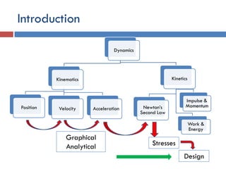
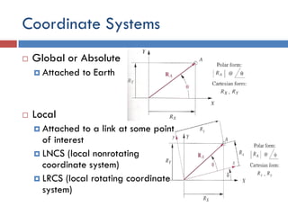
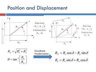
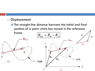
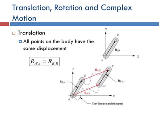
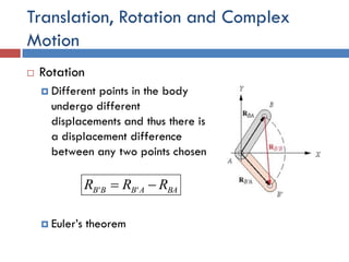
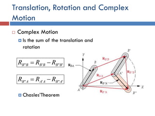
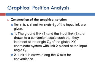
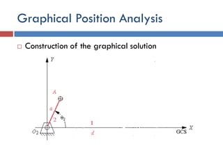
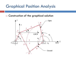
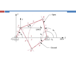
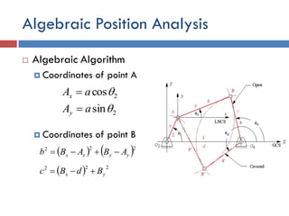
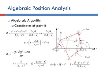
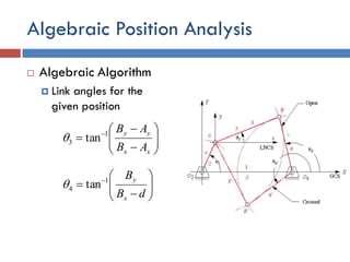
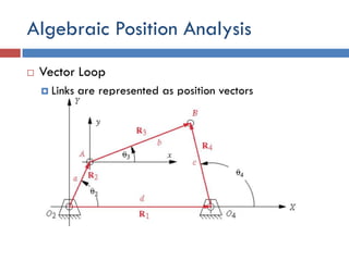
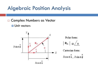
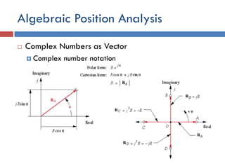
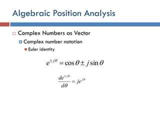
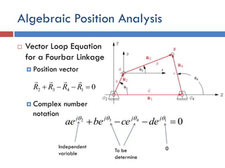
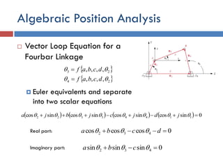
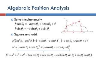
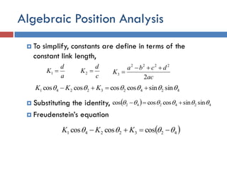
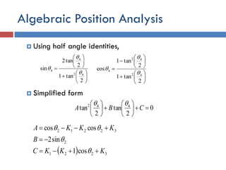
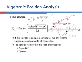
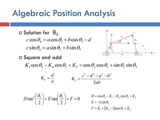
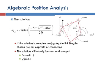
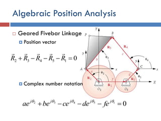
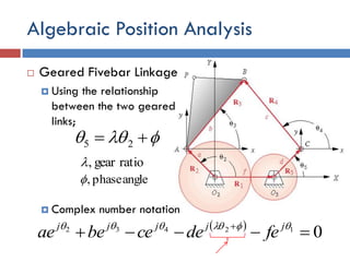
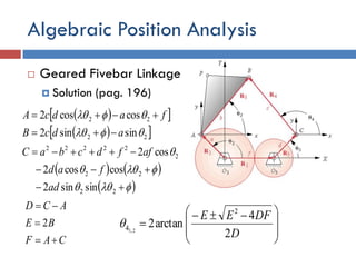
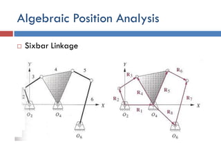
POSITION ANALYSIS
Chapter 4
Introduction
Dynamics
Kinematics
Position Velocity Acceleration
Kinetics
Newton’s
Second Law
Work &
Energy
Impulse &
Momentum
Stresses
Design
Graphical
Analytical
Coordinate Systems
 Global or Absolute
 Attached to Earth
 Local
 Attached to a link at some point
of interest
 LNCS (local nonrotating
coordinate system)
 LRCS (local rotating coordinate
system)
Position and Displacement
22
XYA RRR 






 
X
Y
R
R1
tan
Coordinate
Transformation  sincos yxX RRR 
 cossin yxY RRR 
 Displacement
 The straight-line distance between the initial and final
position of a point which has moved in the reference
frame
ABBA RRR 
Translation, Rotation and Complex
Motion
 Translation
 All points on the body have the
same displacement
BBAA RR '' 
Translation, Rotation and Complex
Motion
 Rotation
 Different points in the body
undergo different
displacements and thus there is
a displacement difference
between any two points chosen
 Euler’s theorem
BAABBB RRR  ''
Translation, Rotation and Complex
Motion
 Complex Motion
 Is the sum of the translation and
rotation
 Chasles’Theorem
'"'" BBBBBB RRR 
'"'" ABAAAB RRR 
Graphical Position Analysis
 For any one-DOF, such a fourbar, only one
parameter is needed to completely define the
positions of all the links. The parameter usually
chosen is the angle of the input link.
Graphical Position Analysis
 Construction of the graphical solution
 The a, b, c, d and the angle θ2 of the input link are
given.
 1. The ground link (1) and the input link (2) are
drawn to a convenient scale such that they
intersect at the origin O2 of the global XY
coordinate system with link 2 placed at the input
angle θ2.
 2. Link 1 is drawn along the X axis for
convenience.
Graphical Position Analysis
 Construction of the graphical solution
Graphical Position Analysis
 Construction of the graphical solution
 3. The compass is set to the scaled length of link
3, and an arc of that radius swung about the end
of link 2 (point A).
Graphical Position Analysis
 Construction of the graphical solution
 4. Set the compass to the scaled length of link 4,
and a second arc swung about the end of link 1
(point O4). These two arcs will have two
intersections at B and B’ that define the two
solution to the position problem for a fourbar
linkage which can be assembled in two
configurations, called circuits, labeled open and
crossed.
 5. The angles of links 3 and 4 can be measured
with a protractor.
Graphical Position Analysis
 Construction of the graphical solution
Algebraic Position Analysis
 Algebraic Algorithm
 Coordinates of point A
 Coordinates of point B
2cosaAx 
2sinaAy 
   222
yyxx ABABb 
  222
yx BdBc 
Algebraic Position Analysis
 Algebraic Algorithm
 Coordinates of point B
     dA
BA
S
dA
BA
dA
dcba
B
x
yy
x
yy
x
x







2
2
2
2
2
2222
02
2
2







 c
dA
BA
SB
x
yy
y
P
PRQQ
By
2
42


 
12
2



dA
A
P
x
y
 
dA
SdA
Q
x
y



2
  22
cSdR 
 dA
dcba
S
x 


2
2222
Algebraic Position Analysis
 Algebraic Algorithm
 Link angles for the
given position








 
xx
yy
AB
AB1
3 tan







 
dB
B
x
y1
4 tan
Algebraic Position Analysis
 Vector Loop
 Links are represented as position vectors
Algebraic Position Analysis
 Complex Numbers as Vector
 Unit vectors
Algebraic Position Analysis
 Complex Numbers as Vector
 Complex number notation
Algebraic Position Analysis
 Complex Numbers as Vector
 Complex number notation
 Euler identity

sincos je j




j
j
je
d
de


Algebraic Position Analysis
 Vector Loop Equation
for a Fourbar Linkage
 Position vector
 Complex number
notation
01432  RRRR

01432
  jjjj
decebeae
0Independent
variable
To be
determine
Algebraic Position Analysis
 Vector Loop Equation for a
Fourbar Linkage
 Euler equivalents and separate
into two scalar equations
 
 24
23
,,,,
,,,,


dcbaf
dcbaf


        0sincossincossincossincos 11443322   jdjcjbja
Real part: 0coscoscos 432  dcba 
0sinsinsin 432   cbaImaginary part:
Algebraic Position Analysis
 Solve simultaneously
 Square and add
dcab  423 coscoscos 
423 sinsinsin  cab 
     2
42
2
423
2
3
22
coscossinsincossin dcacab  
   2
42
2
42
2
coscossinsin dcacab  
 424242
2222
coscossinsin2cos2cos2   accdaddcab
Algebraic Position Analysis
 To simplify, constants are define in terms of the
constant link length,
 Substituting the identity,
 Freudenstein’s equation
a
d
K 1
424232241 sinsincoscoscoscos   KKK
c
d
K 2
ac
dcba
K
2
2222
3


  424242 sinsincoscoscos  
 4232241 coscoscos   KKK
Algebraic Position Analysis
 Using half angle identities,
 Simplified form














2
tan1
2
tan2
sin
42
4
4


















2
tan1
2
tan1
cos
42
42
4



0
2
tan
2
tan 442












CBA

  3221
2
32212
cos1
sin2
coscos
KKKC
B
KKKA






Algebraic Position Analysis
 The solution,
 If the solution is complex conjugate, the link lengths
chosen are not capable of connection
 The solution will usually be real and unequal
 Crossed (+)
 Open (-)
A
ACBB
2
4
2
tan
2
4 













 

A
ACBB
2
4
arctan2
2
4 2,1

Algebraic Position Analysis
 Solution for θ3
 Square and add
dbac  324 coscoscos 
324 sinsinsin  bac 
323252431 sinsincoscoscoscos   KKK
b
d
K 4
ab
badc
K
2
2222
5


0
2
tan
2
tan 332












FED

  5241
2
52412
cos1
sin2
coscos
KKKF
E
KKKD






Algebraic Position Analysis
 The solution,
 If the solution is complex conjugate, the link lengths
chosen are not capable of connection
 The solution will usually be real and unequal
 Crossed (+)
 Open (-)







 

D
DFEE
2
4
arctan2
2
3 2,1

Algebraic Position Analysis
 Fourbar Slider-Crank
Linkage
 Position vector
 Complex number
notation
01432  RRRR

01432
  jjjj
decebeae
0Independent
variable
To be
determine
Algebraic Position Analysis
 Vector Loop Equation for a
Fourbar Linkage
 Euler equivalents and separate
into two scalar equations
        0sincossincossincossincos 11443322   jdjcjbja
Real part: 0coscoscos 432  dcba 
0sinsinsin 432   cbaImaginary part:
Algebraic Position Analysis
 The solution,
32
2
3
coscos
sin
arcsin1



bad
b
ca






 



 




 

b
ca 2
3
sin
arcsin2
Algebraic Position Analysis
 Inverted Slider-Crank (p193-p194)
Algebraic Position Analysis
 Geared Fivebar Linkage
 Position vector
 Complex number notation
015432  RRRRR

015432
  jjjjj
fedecebeae
Algebraic Position Analysis
 Geared Fivebar Linkage
 Using the relationship
between the two geared
links;
 Complex number notation
  25
 
012432
   jjjjj
fedecebeae
ratiogear,
anglephase,
Algebraic Position Analysis
 Geared Fivebar Linkage
 Solution (pag. 196)







 

D
DFEE
2
4
arctan2
2
4 2,1

  
  
   
 









22
22
2
22222
22
22
sinsin2
coscos2
cos2
sinsin2
coscos2
ad
fad
affdcbaC
adcB
fadcA
CAF
BE
ACD



2
Algebraic Position Analysis
 Geared Fivebar Linkage
 Solution (pag. 196)







 

L
LNMM
2
4
arctan2
2
3 2,1

  
  
   
 









22
22
2
22222
22
22
sinsin2
coscos2
cos2
sinsin2
coscos2
ad
fad
affdcbaK
dabH
fdabG
KGN
HM
GKL



2
Algebraic Position Analysis
 Sixbar Linkage
Algebraic Position Analysis
 Sixbar Linkage

Ch04 position analysis

  • 1.
  • 2.
    Introduction Dynamics Kinematics Position Velocity Acceleration Kinetics Newton’s SecondLaw Work & Energy Impulse & Momentum Stresses Design Graphical Analytical
  • 3.
    Coordinate Systems  Globalor Absolute  Attached to Earth  Local  Attached to a link at some point of interest  LNCS (local nonrotating coordinate system)  LRCS (local rotating coordinate system)
  • 4.
    Position and Displacement 22 XYARRR          X Y R R1 tan Coordinate Transformation  sincos yxX RRR   cossin yxY RRR 
  • 5.
     Displacement  Thestraight-line distance between the initial and final position of a point which has moved in the reference frame ABBA RRR 
  • 6.
    Translation, Rotation andComplex Motion  Translation  All points on the body have the same displacement BBAA RR '' 
  • 7.
    Translation, Rotation andComplex Motion  Rotation  Different points in the body undergo different displacements and thus there is a displacement difference between any two points chosen  Euler’s theorem BAABBB RRR  ''
  • 8.
    Translation, Rotation andComplex Motion  Complex Motion  Is the sum of the translation and rotation  Chasles’Theorem '"'" BBBBBB RRR  '"'" ABAAAB RRR 
  • 9.
    Graphical Position Analysis For any one-DOF, such a fourbar, only one parameter is needed to completely define the positions of all the links. The parameter usually chosen is the angle of the input link.
  • 10.
    Graphical Position Analysis Construction of the graphical solution  The a, b, c, d and the angle θ2 of the input link are given.  1. The ground link (1) and the input link (2) are drawn to a convenient scale such that they intersect at the origin O2 of the global XY coordinate system with link 2 placed at the input angle θ2.  2. Link 1 is drawn along the X axis for convenience.
  • 11.
    Graphical Position Analysis Construction of the graphical solution
  • 12.
    Graphical Position Analysis Construction of the graphical solution  3. The compass is set to the scaled length of link 3, and an arc of that radius swung about the end of link 2 (point A).
  • 13.
    Graphical Position Analysis Construction of the graphical solution  4. Set the compass to the scaled length of link 4, and a second arc swung about the end of link 1 (point O4). These two arcs will have two intersections at B and B’ that define the two solution to the position problem for a fourbar linkage which can be assembled in two configurations, called circuits, labeled open and crossed.  5. The angles of links 3 and 4 can be measured with a protractor.
  • 14.
    Graphical Position Analysis Construction of the graphical solution
  • 16.
    Algebraic Position Analysis Algebraic Algorithm  Coordinates of point A  Coordinates of point B 2cosaAx  2sinaAy     222 yyxx ABABb    222 yx BdBc 
  • 17.
    Algebraic Position Analysis Algebraic Algorithm  Coordinates of point B      dA BA S dA BA dA dcba B x yy x yy x x        2 2 2 2 2 2222 02 2 2         c dA BA SB x yy y P PRQQ By 2 42     12 2    dA A P x y   dA SdA Q x y    2   22 cSdR   dA dcba S x    2 2222
  • 18.
    Algebraic Position Analysis Algebraic Algorithm  Link angles for the given position           xx yy AB AB1 3 tan          dB B x y1 4 tan
  • 19.
    Algebraic Position Analysis Vector Loop  Links are represented as position vectors
  • 20.
    Algebraic Position Analysis Complex Numbers as Vector  Unit vectors
  • 21.
    Algebraic Position Analysis Complex Numbers as Vector  Complex number notation
  • 22.
    Algebraic Position Analysis Complex Numbers as Vector  Complex number notation  Euler identity  sincos je j     j j je d de  
  • 23.
    Algebraic Position Analysis Vector Loop Equation for a Fourbar Linkage  Position vector  Complex number notation 01432  RRRR  01432   jjjj decebeae 0Independent variable To be determine
  • 24.
    Algebraic Position Analysis Vector Loop Equation for a Fourbar Linkage  Euler equivalents and separate into two scalar equations    24 23 ,,,, ,,,,   dcbaf dcbaf           0sincossincossincossincos 11443322   jdjcjbja Real part: 0coscoscos 432  dcba  0sinsinsin 432   cbaImaginary part:
  • 25.
    Algebraic Position Analysis Solve simultaneously  Square and add dcab  423 coscoscos  423 sinsinsin  cab       2 42 2 423 2 3 22 coscossinsincossin dcacab      2 42 2 42 2 coscossinsin dcacab    424242 2222 coscossinsin2cos2cos2   accdaddcab
  • 26.
    Algebraic Position Analysis To simplify, constants are define in terms of the constant link length,  Substituting the identity,  Freudenstein’s equation a d K 1 424232241 sinsincoscoscoscos   KKK c d K 2 ac dcba K 2 2222 3     424242 sinsincoscoscos    4232241 coscoscos   KKK
  • 27.
    Algebraic Position Analysis Using half angle identities,  Simplified form               2 tan1 2 tan2 sin 42 4 4                   2 tan1 2 tan1 cos 42 42 4    0 2 tan 2 tan 442             CBA    3221 2 32212 cos1 sin2 coscos KKKC B KKKA      
  • 28.
    Algebraic Position Analysis The solution,  If the solution is complex conjugate, the link lengths chosen are not capable of connection  The solution will usually be real and unequal  Crossed (+)  Open (-) A ACBB 2 4 2 tan 2 4                  A ACBB 2 4 arctan2 2 4 2,1 
  • 29.
    Algebraic Position Analysis Solution for θ3  Square and add dbac  324 coscoscos  324 sinsinsin  bac  323252431 sinsincoscoscoscos   KKK b d K 4 ab badc K 2 2222 5   0 2 tan 2 tan 332             FED    5241 2 52412 cos1 sin2 coscos KKKF E KKKD      
  • 30.
    Algebraic Position Analysis The solution,  If the solution is complex conjugate, the link lengths chosen are not capable of connection  The solution will usually be real and unequal  Crossed (+)  Open (-)           D DFEE 2 4 arctan2 2 3 2,1 
  • 31.
    Algebraic Position Analysis Fourbar Slider-Crank Linkage  Position vector  Complex number notation 01432  RRRR  01432   jjjj decebeae 0Independent variable To be determine
  • 32.
    Algebraic Position Analysis Vector Loop Equation for a Fourbar Linkage  Euler equivalents and separate into two scalar equations         0sincossincossincossincos 11443322   jdjcjbja Real part: 0coscoscos 432  dcba  0sinsinsin 432   cbaImaginary part:
  • 33.
    Algebraic Position Analysis The solution, 32 2 3 coscos sin arcsin1    bad b ca                     b ca 2 3 sin arcsin2
  • 34.
    Algebraic Position Analysis Inverted Slider-Crank (p193-p194)
  • 35.
    Algebraic Position Analysis Geared Fivebar Linkage  Position vector  Complex number notation 015432  RRRRR  015432   jjjjj fedecebeae
  • 36.
    Algebraic Position Analysis Geared Fivebar Linkage  Using the relationship between the two geared links;  Complex number notation   25   012432    jjjjj fedecebeae ratiogear, anglephase,
  • 37.
    Algebraic Position Analysis Geared Fivebar Linkage  Solution (pag. 196)           D DFEE 2 4 arctan2 2 4 2,1                       22 22 2 22222 22 22 sinsin2 coscos2 cos2 sinsin2 coscos2 ad fad affdcbaC adcB fadcA CAF BE ACD    2
  • 38.
    Algebraic Position Analysis Geared Fivebar Linkage  Solution (pag. 196)           L LNMM 2 4 arctan2 2 3 2,1                       22 22 2 22222 22 22 sinsin2 coscos2 cos2 sinsin2 coscos2 ad fad affdcbaK dabH fdabG KGN HM GKL    2
  • 39.
  • 40.