ec.diferenciales lista 2

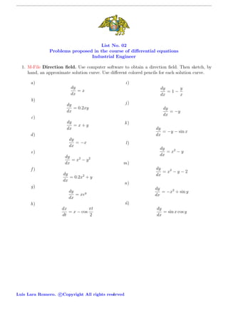
1. List No. 02
Problems proposed in the course of differential equations
Industrial Engineer
1. M-File Direction field. Use computer software to obtain a direction field. Then sketch, by
hand, an approximate solution curve. Use different colored pencils for each solution curve.
a)
dy
dx
= x
b)
dy
dx
= 0.2xy
c)
dy
dx
= x + y
d)
dy
dx
= −x
e)
dy
dx
= x2
− y2
f )
dy
dx
= 0.2x2
+ y
g)
dy
dx
= xey
h)
dx
dt
= x − cos
πt
2
i)
dy
dx
= 1 −
y
x
j)
dy
dx
= −y
k)
dy
dx
= −y − sin x
l)
dy
dx
= x2
− y
m)
dy
dx
= x2
− y − 2
n)
dy
dx
= −x2
+ sin y
˜n)
dy
dx
= sin x cos y
Luis Lara Romero. c⃝Copyright All rights reserved1

2. 2. M-File. Make a computer program to generate the graphs of the following curves. Use the plot
command of MATLAB
a) y = xe−x2
, x ∈ [−3, 3]
b) y = e−x
sin x, x ∈ [0, 2π]
c) x = 1 +
1
2
e−0,08t
sin(
1
2
πt), t ∈ [0, 10π]
d) x = e−2t
(4 cos 3t + 5 sin 3t), t ∈ [0, 4π]
3. M-File. Make a computer program to generate the graphs of the following curves. Use the
ezplot command of MATLAB
a) (x2
+ y2
− 1)3
= x2
y3
b) (x2
+ y2
)2
= 2x(x2
− 3y2
)
c) x2
− 2y3
+ 4y = 2
d) 3(x2
+ y2
)2
= 100xy
e) x2
(x2
+ y2
) = y2
f ) x2
y2
+ xy = 2
4. M-File. Make a computer program to generate the graphs of the following curves. Use the
ezplot command of MATLAB
a) 2 + y2
= c(4 + x2
), c = 1, 2, 3, 4, 5
b) y = −
1
cos(x) + c
, c = −2, −1, 0, 1, 2
c) x cos(
y
x
) = c, c = −2, −1, 0, 1, 2
d) x4
= c(x2
− y2
), c = 1, 2, 3
Luis Lara Romero. c⃝Copyright All rights reserved2