Download as PDF, PPTX

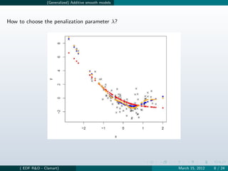
![(Generalized) Additive smooth models
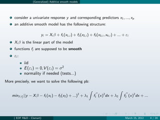
Ordinary Cross Validation
leave one observation yi
estimate a model µ−i on the new data set
forecast yi with µ−i
i
do that for all i
choose the λ that minimizes the OCV score:
n
V0 (λ) = (yi − µ−i )2 /n
i
i=1
Pb: calculation time
Generalized Cross Validation [Craven and Wahba (1979)]
Vg (λ) = n y − X βλ |2 /(n − tr (Fλ ))2
Advantages of GCV:
λ is obtained by numerical minimization of Vg (few comp. cost)
Vg (λ) is invariant when doing useful transf. of the data (on-line update, big data)
⇒ Software: R, package mgcv (see[Wood (2001)] and [Wood (2006)])
( EDF R&D - Clamart) March 15, 2012 9 / 24](https://image.slidesharecdn.com/adaptivegam-120318192404-phpapp02/85/Prevision-de-consommation-electrique-avec-adaptive-GAM-9-320.jpg)
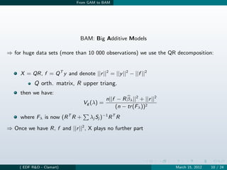
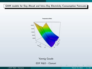
![From GAM to BAM
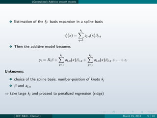
⇒ Application for large data sets:
X0 y0
X is too big and has to be split: , similarly y =
X1 y1
R0
form QR dec. X 0 = Q0 X0 and = Q1 R see section 12.5 of
X1
[Golub and Van Loan (1996)]
T
Q0 0 Q0 y0
then X = QR with Q = Q1 and Q T y = Q1
T
0 I y1
⇒ On-line update
X0 , y0 past data, X1 , y1 last observations
Use the new data X1 , y1 to update R, f and ||r ||2
Re-estimate λ and βλ (previous values can be used as starting values for the
numerical optimization)
( EDF R&D - Clamart) March 15, 2012 11 / 24](https://image.slidesharecdn.com/adaptivegam-120318192404-phpapp02/85/Prevision-de-consommation-electrique-avec-adaptive-GAM-11-320.jpg)
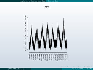
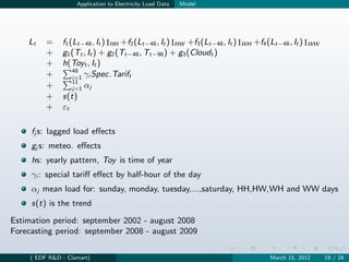
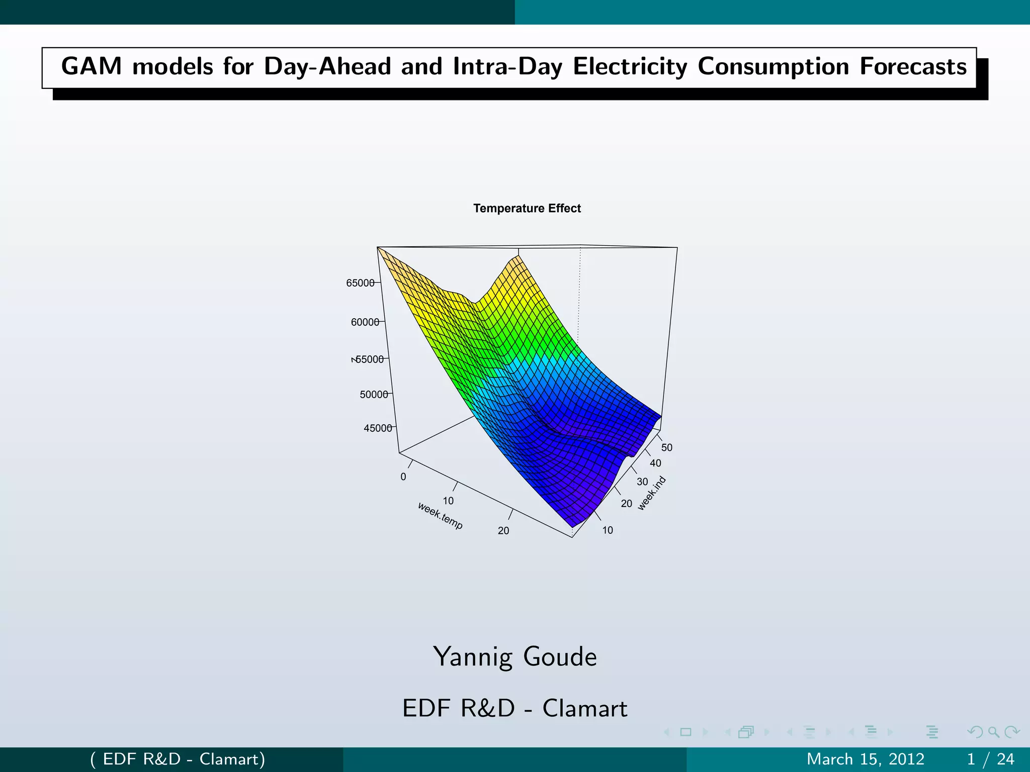
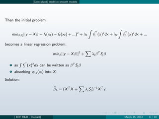
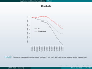
![Application to Electricity Load Data Model
GAM Model
10000
Temperature Effect
5000
70000
65000
Load (MW)
0
L[t]
60000
−5000
55000
50000 40
30 30
−10000
20 20
I[t]
T[t 10 Mo Fr Su
] 10
0 we Sa
0
0 10 20 30 40
Hour
Yearly Cycle Trend
10000
80000
70000
5000
60000
z
0
50000
40000
−5000
40
0.0 30
0.2
0.4 20
nt
Po
sta
san 0.6
In
10
−10000
0.8
0
120000 140000 160000 180000 200000 220000 240000
t
( EDF R&D - Clamart) March 15, 2012 20 / 24](https://image.slidesharecdn.com/adaptivegam-120318192404-phpapp02/85/Prevision-de-consommation-electrique-avec-adaptive-GAM-20-320.jpg)
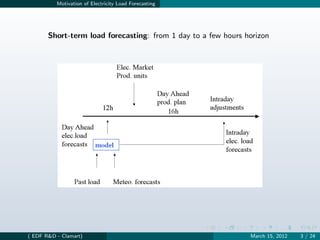
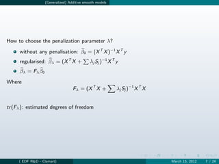
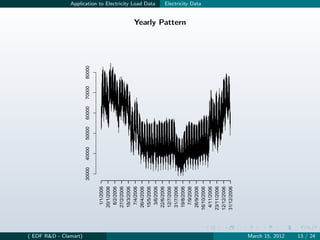
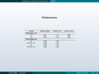
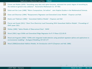
![Application to Electricity Load Data Model
Lagged Load Effect, WW Lagged Load Effect, WH
80000
70000
70000
60000
L[t]
60000
L[t]
50000
50000
40000
40000
40 30000 40
80000 30 80000 30
70000 20 70000 20
60000 60000
]
]
I[t
I[t
L[t 50000 10 L[t 50000 10
−1 −1
] 40000 ] 40000
30000 0 30000 0
Lagged Load Effect, HW Lagged Load Effect, HH
30000
20000
80000
L[t]
10000
L[t]
60000 0
−10000
40000
40 40
80000 30 80000 30
70000 20 70000 20
60000 60000
]
]
I[t
I[t
L[t 50000 10 L[t 50000 10
−1 −1
] 40000 ] 40000
30000 0 30000 0
( EDF R&D - Clamart) March 15, 2012 21 / 24](https://image.slidesharecdn.com/adaptivegam-120318192404-phpapp02/85/Prevision-de-consommation-electrique-avec-adaptive-GAM-21-320.jpg)

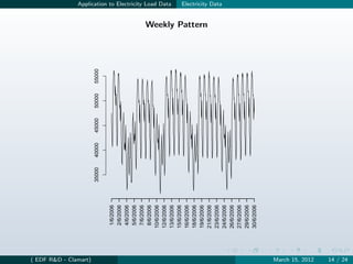
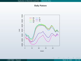
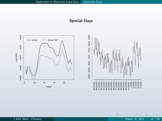
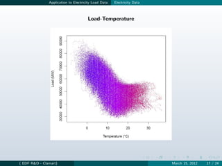
The document discusses generalized additive models (GAM) for short-term electricity load forecasting. GAMs are smooth additive models that decompose a response variable into additive components like trends, cyclic patterns, and nonlinear effects. They summarize how GAMs can model various drivers of electricity consumption, including temperature effects, day-of-week patterns, and lagged load values. Big additive models (BAM) allow applying GAMs to large electricity load datasets. BAMs use QR decomposition and online updating to efficiently estimate high-dimensional additive models.


![11.[104 111]analytical solution for telegraph equation by modified of sumudu ...](https://cdn.slidesharecdn.com/ss_thumbnails/11-104-111analyticalsolutionfortelegraphequationbymodifiedofsumudutransformelzakitransform-120513000219-phpapp01-thumbnail.jpg?width=640&height=640&fit=bounds)