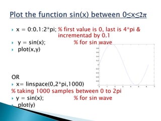
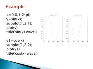
This document provides code examples for creating different types of plots in MATLAB, including line plots, bar plots, polar plots, and pie charts. It shows how to generate a sine wave plot and customize it by adding titles, labels, legends and adjusting axes. It also demonstrates how to create subplot layouts to show multiple graphs together and explores functions like bar, stairs, compass and pie for generating other common plot types from data.

1. Miss. Patil Apurva Pandurang
M.Tech (Electronics)
1

2.  x = 0:0.1:2*pi; % first value is 0, last is 2*pi &
incrementad by 0.1
 y = sin(x); % for sin wave
 plot(x,y)
OR
 x= linspace(0,2*pi,1000)
% taking 1000 samples between 0 to 2pi
 y = sin(x); % for sin wave
 plot(y)
0 1 2 3 4 5 6 7
-1
-0.8
-0.6
-0.4
-0.2
0
0.2
0.4
0.6
0.8
1
2

3.  plot(.)
>> x=linspace(0,2*pi,50);
>>y=sin(x);
>>plot(y)
 stem(.)
>> x=linspace(0,2*pi,50);
>>y=sin(x);
>>stem(y)
0 5 10 15 20 25 30 35 40 45 50
-1
-0.8
-0.6
-0.4
-0.2
0
0.2
0.4
0.6
0.8
1
0 5 10 15 20 25 30 35 40 45 50
-1
-0.8
-0.6
-0.4
-0.2
0
0.2
0.4
0.6
0.8
1
3

4.  title(.)
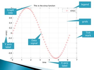
>>title(‘This is the sinus function’)
 xlabel(.)
>>xlabel(‘time’)
 ylabel(.)
>>ylabel(‘sin(x)’)
 legend(.)
>>legend ('sin_x')
 grid
>> grid on
>> grid off
 axis([xmin xmax ymin ymax])
Sets the minimum and maximum limits of the x- and y-axes
0 1 2 3 4 5 6 7
-1
-0.8
-0.6
-0.4
-0.2
0
0.2
0.4
0.6
0.8
1
time
sin(x)
This is the sinus function
sin(x)
4

5. 0 1 2 3 4 5 6 7
-1
-0.8
-0.6
-0.4
-0.2
0
0.2
0.4
0.6
0.8
1
time
sin(x) This is the sinus function
sin(x)
Data
signal
X axis
label
grids
Tick
mark
legend
Graph
title
Y axis
label
5

6.  Multiple x-y pair arguments create multiple
graph
x = 0:pi/100:2*pi;
y = sin(x);
y2 = sin(x-0.25);
y3 = sin(x-0.5);
plot(x,y,x,y2,x,y3)
0 1 2 3 4 5 6 7
-1
-0.8
-0.6
-0.4
-0.2
0
0.2
0.4
0.6
0.8
1
6

7.  plot(x,y,’line specifiers’)
Define style, color of line
& type of marker
7

8. Line Specifies Line Specifies Marker Specifies
Style Color Type
Solid - red r plus sign +
dotted : green g circle o
dashed -- blue b asterisk *
dash-dot -. Cyan c point .
magenta m square s
yellow y diamond d
black k
0 1 2 3 4 5 6 7
-1
-0.8
-0.6
-0.4
-0.2
0
0.2
0.4
0.6
0.8
1
Example:
x=0:0.1:2*pi;
y=sin(x);
plot(x,y,'r-*')
8

9.  fplot(‘function’,[limits])
E.g.
Plot the equation
x^3-2*cos(0.66*x)+4*sin(2*x)-1 in the limit
between -3 & 3
>>fplot('x^3-2*cos(0.66*x)+4*sin(2*x)-1', [-3 3])
-3 -2 -1 0 1 2 3
-30
-20
-10
0
10
20
30
9

10. Subplots
 subplot(m,n,P)
rows
columns
position
x=0:0.1:2*pi;
y=sin(x);
subplot(2,1,1);
plot(y)
title('sin(x) wave')
y1=cos(x)
subplot(2,1,2);
plot(y1)
title('cos(x) wave')
0 10 20 30 40 50 60 70
-1
-0.5
0
0.5
1
sin(x) wave
0 10 20 30 40 50 60 70
-1
-0.5
0
0.5
1
cos(x) wave
10

11. 0 20 40 60 80
-1
-0.8
-0.6
-0.4
-0.2
0
0.2
0.4
0.6
0.8
1
sin(x) wave
0 20 40 60 80
-1
-0.8
-0.6
-0.4
-0.2
0
0.2
0.4
0.6
0.8
1
cos(x) wavex=0:0.1:2*pi;
y=sin(x);
subplot(1,2,1);
plot(y)
title('sin(x) wave')
y1=cos(x)
subplot(1,2,2);
plot(y1)
title('cos(x) wave')
Example
11

12. Example:
x=0:0.1:4*pi;
y=sin(x);
subplot(2,2,1);
plot(y)
title('sin(x) wave')
y1=cos(x)
subplot(2,2,2);
plot(y1)
title('cos(x) wave')
y2=sawtooth(x)
subplot(2,2,3);
plot(y2)
title('sawtooth wave')
y3=rand(4)
subplot(2,2,4);
plot(y3)
title('randam wave')
0 50 100 150
-1
-0.5
0
0.5
1
sin(x) wave
0 50 100 150
-1
-0.5
0
0.5
1
cos(x) wave
0 50 100 150
-1
-0.5
0
0.5
1
sawtooth wave
1 2 3 4
0
0.5
1
randam wave
12

13. Example
clc
clear all
x=0:0.1:4*pi;
y=sin(x);
subplot(2,2,1:2);
plot(y)
title('sin(x) wave')
y2=sawtooth(x)
subplot(2,2,3);
plot(y2)
title('sawtooth wave')
y3=rand(4)
subplot(2,2,4);
plot(y3)
title('randam wave')
0 50 100 150
-1
-0.5
0
0.5
1
sawtooth wave
1 2 3 4
0
0.5
1
randam wave
0 20 40 60 80 100 120 140
-1
-0.5
0
0.5
1
sin(x) wave
13

14.  bar(x,y)
x=[1 2 3 4 5]
y=[1 2 3 4 5]
bar(x,y)
 function creates
vertical Bar plot 1 2 3 4 5
0
0.5
1
1.5
2
2.5
3
3.5
4
4.5
5
14

15.  barh(x,y)
x=[1 2 3 4 5]
y=[1 2 3 4 6]
barh(x,y)
 function creates
horizontal Bar plot
0 1 2 3 4 5 6
1
2
3
4
5
15

16.  stairs(x,y)
x=[0 1 2 3 4]
y=[1 2 3 4 6]
stairs(x,y)
 function creates
stair plot
0 0.5 1 1.5 2 2.5 3 3.5 4
1
1.5
2
2.5
3
3.5
4
4.5
5
5.5
6
16

17.  compass(x,y)
x=[1 2 3 4 5]
y=[1 2 3 4 6]
compass(x,y)
 function creates polar plot
Location of points to plot in
“Cartesian coordinates”
2
4
6
8
30
210
60
240
90
270
120
300
150
330
180 0
17

18.  pie(x)
x=[1 2 3 4 5]
pie(x)
 function creates pie plot
 Values are in terms of percentage
7%
13%
20%
27%
33%
18

19. Thank you…..
19