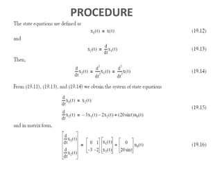
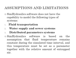
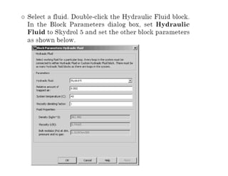
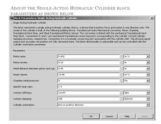
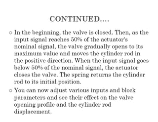
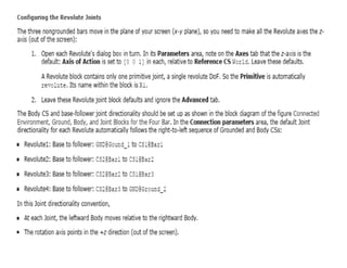
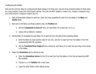
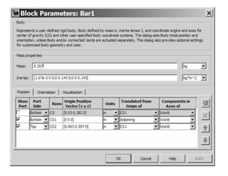
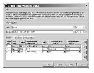
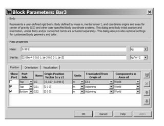
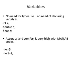
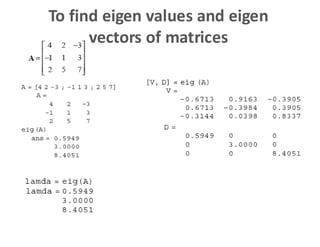
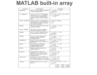
Variables
• No needfor types. i.e., no need of declaring
variables
int a;
double b;
float c;
• Accuracy and comfort is very high with MATLAB
codes.
>>x=5;
>>x1=2;
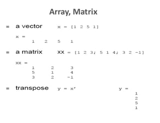
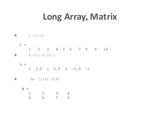
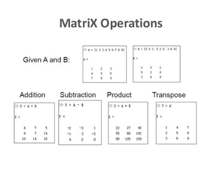
Matrixes and vectors
•x = [1,2,3] , vector-row,
• y=[1;2;3], vector-column,
• x=0:0.1:0.8 , vector x=[0,0.1,0.2,0.3....0.8],
• A = [1,3,5;5,6,7;8,9,10], matrix,
• A(1,2), element of matrix, 1. row, 2. column,
• A(:,2), second column of matrix,
• A(1,:), first row of matrix ,
• C=[A;[10,20,30]] matrix with additional row,
• B=A(2:3,1:2), part of matrix,
• x’, transpose.
46
10.
Matrixes and vectors
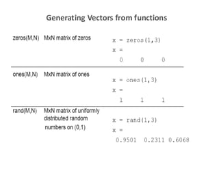
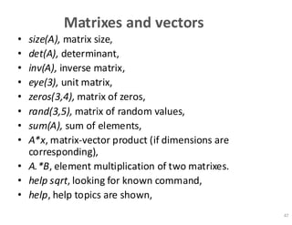
•size(A), matrix size,
• det(A), determinant,
• inv(A), inverse matrix,
• eye(3), unit matrix,
• zeros(3,4), matrix of zeros,
• rand(3,5), matrix of random values,
• sum(A), sum of elements,
• A*x, matrix-vector product (if dimensions are
corresponding),
• A.*B, element multiplication of two matrixes.
• help sqrt, looking for known command,
• help, help topics are shown,
47
11.
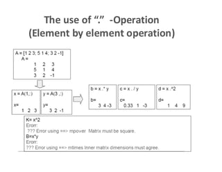
The use of“.” -Operation
(Element by element operation)
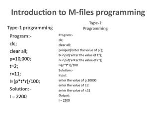
Introduction to M-filesprogramming
Program:-
clc;
clear all;
p=10,000;
t=2;
r=11;
I=(p*t*r)/100;
Solution:-
I = 2200
Program:-
clc;
clear all;
p=input('enter the value of p:');
t=input('enter the value of t:');
r=input('enter the value of r:');
I=(p*t*r)/100
Solution:-
Input:
enter the value of p:10000
enter the value of t:2
enter the value of r:11
Output:
I = 2200
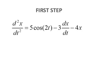
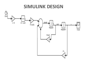
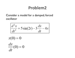
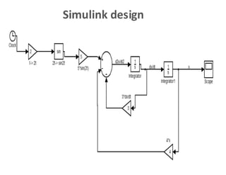
Type-1 programming
Type-2
Programming
14.
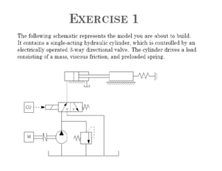
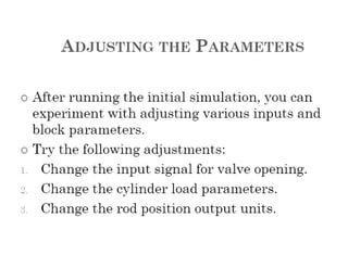
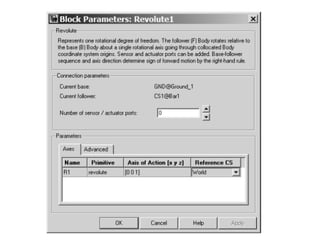
Solving Nonlinear Equationsby
Function
nle.m (function of the program)
function f = nle(x)
f(1) = x(1)-4*x(1)*x(1)-x(1)*x(2);
f(2) = 2*x(2)-x(2)*x(2)+3*x(1)*x(2);
Main body of the Program:-
x0 = [1 1]';
x = fsolve('nle', x0)
Solution of the program:-
x =
0.2500
0.0000
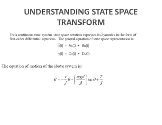
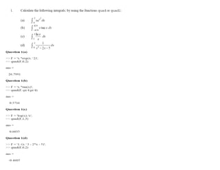
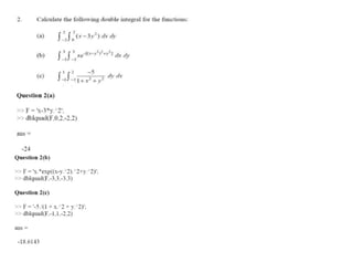
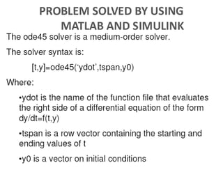
Numerical Integration
• Numericalintegration of the integral f (x) dx is called quadrature. MATLAB
provides the following built-in functions for numerical integration:
quad:
• It integrates the specified function over specified limits, based on adaptive
Simpson's rule.
• The general call syntax for both quad and quadl is as follows:
Syntax:-
integral = quad(‘function’, a, b)
dblquad: (It calculates double integration)
• MATLAB provides a function dblquad. The calling syntax for dblquad is:
Syntax:-
I = dblquad(‘function_xy’, xmin, xmax, ymin, ymax)
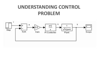
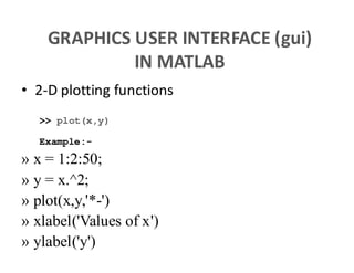
GRAPHICS USER INTERFACE(gui)
IN MATLAB
• 2-D plotting functions
>> plot(x,y)
Example:-
» x = 1:2:50;
» y = x.^2;
» plot(x,y,'*-')
» xlabel('Values of x')
» ylabel('y')
26.
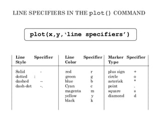
LINE SPECIFIERS INTHE plot() COMMAND
Line Specifier Line Specifier Marker Specifier
Style Color Type
Solid - red r plus sign +
dotted : green g circle o
dashed -- blue b asterisk *
dash-dot -. Cyan c point .
magenta m square s
yellow y diamond d
black k
plot(x,y,‘line specifiers’)
27.
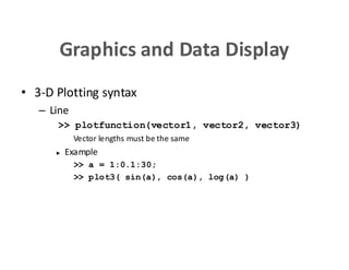
Graphics and DataDisplay
• 3-D Plotting syntax
– Line
>> plotfunction(vector1, vector2, vector3)
Vector lengths must be the same
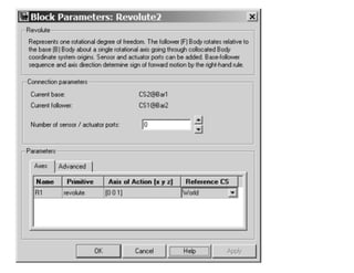
► Example
>> a = 1:0.1:30;
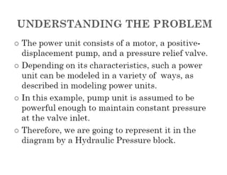
>> plot3( sin(a), cos(a), log(a) )
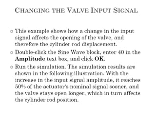
ØPlot of thesine function from limits of 0 to (2* pi).
Program:-
clear all; % clear all variables
clc; % clear screen
N=30;
h=pi/N;
x=0:h:(2*pi);
y=sin(x);
plot(x,y)
xlabel('x')
ylabel('sin(x')
title('Graph of sine function in 0 to (2*pi) range')
0 1 2 3 4 5 6 7
-1
-0.8
-0.6
-0.4
-0.2
0
0.2
0.4
0.6
0.8
1
x
sin(x)
Graph of sine function in 0 to (2*pi) range
sin(x)
Hint: - Direct plotting of curves can be done by ‘fplot’ command also
Syntax: fplot (‘function’, *lower limit, upper limit)
fplot ('x*cos(x)',[0, 10*pi]);
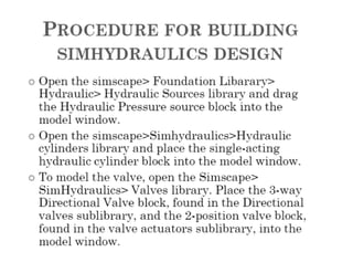
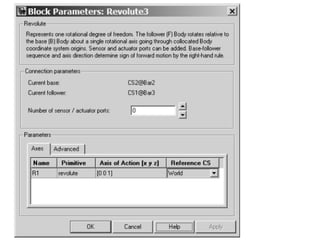
33.
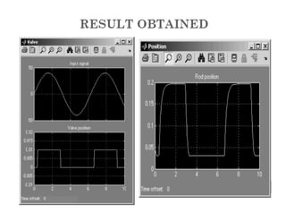
Ø To plotthe function y(x)= -3*x+4 from limits -1 to 2.
Program:-
clc;
clear all;
x=-1:1:2;
y=-3*x+4;
figure
plot(x,y)
xlabel('x')
ylabel('y=f(x)')
grid on
title('plot of function f_1(x)');
legend('f_1(x)');
axis([-2 4 -2 12])
-2 -1 0 1 2 3 4
-2
0
2
4
6
8
10
12
x
y=f(x)
plot of function f1
(x)
f1
(x)
34.
ØPlotting multiple plotsin same window, for example plotting
sine curve and cosine curve in single window.
Program:-
clc;
clear all;
N=15;
h=pi/N;
x=0:h:2*pi;
plot(x,sin(x),'r-',x,cos(x),'g--')
legend('sine','cosine');
grid
xlabel('x');
ylabel('functions');
title('Test of multi-plot option in Matlab');
0 1 2 3 4 5 6 7
-1
-0.8
-0.6
-0.4
-0.2
0
0.2
0.4
0.6
0.8
1
x
func
tions
Test of multi-plot option in Matlab
sine
cosine
35.
ØComparing multiple plotsin single window for example
y1 = 2 cos(x), y2 = cos(x), and y3 =0.5* cos(x), in the interval 0≤ x≤ (2*pi)
Program:-
x = 0:pi/100:2*pi;
y1 = 2*cos(x);
y2 = cos(x);
y3 = 0.5*cos(x);
plot(x,y1,'--',x,y2,'-',x,y3,':');
xlabel('0 leq x leq 2pi');
ylabel('Cosine functions');
legend('2*cos(x)','cos(x)','0.5*cos(x)');
title('Typical example of multiple plots');
axis([0 2*pi -3 3]);
0 1 2 3 4 5 6
-3
-2
-1
0
1
2
3
0 £ x £ 2p
Cosine
func
tions
Typical example of multiple plots
2*cos(x)
cos (x)
0.5*cos(x)
36.
ØTo plot thecurve of exponential of x and sin(x) in a single
window
Program:-
clc;
clear all;
x=0:.1:2*pi;
y=sin(x);
plot(x,y);
grid on;
hold on;
plot(x, exp(-x), 'r:*');
axis([0 2*pi 0 1]);
title('2-D Plot');
xlabel('Time');
ylabel('Sin(t) ');
text(pi/3, sin(pi/3), '<--sin(pi/3) ');
legend('Sine Wave','Decaying Exponential');
0 1 2 3 4 5 6
0
0.1
0.2
0.3
0.4
0.5
0.6
0.7
0.8
0.9
1
2-D Plot
Time
Sin
(t)
<--sin(p/3)
Sine Wave
Decaying Exponential
Ø Plot thesurface defined by the function
f(x,y)= (x-3)2 – (y-2)2 on the domain -2 ≤ x ≤ 4 and 1 ≤ y ≤ 3.
Program:-
clc;
clear all;
[X,Y] = meshgrid(-2:0.2:4,1:0.2:3);
Z = (X-3).^2 - (Y-2).^2;
mesh(X,Y,Z);
xlabel('x');
ylabel('y');
-2
0
2
4
1
1.5
2
2.5
3
-5
0
5
10
15
20
25
x
y
43.
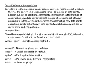
Curve Fitting andInterpolation
Curve fitting is the process of constructing a curve, or mathematical function,
that has the best fit (in a least square sense) to a series of data points,
possibly subject to additional constraints. Interpolation is the method of
constructing new data points within the range of a discrete set of known
data points. Extrapolation is the process of constructing new data points
outside a discrete set of known data points. Matlab has many utilities for
curve fitting and interpolation.
Interpolation:-
Given the data points (xi, yi), find yj at desired xj ≠ xi from yj = f(xj), where f is
a continuous function to be found from interpolation.
Syntax:- ynew = interp1(x,y,xnew, method ).
’nearest’-> Nearest neighbor interpolation
’linear’ -> Linear interpolation (default)
’spline’ -> Cubic spline interpolation
’pchip’ -> Piecewise cubic Hermite interpolation
’cubic’ -> Same as ’pchip’
44.
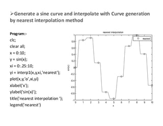
ØGenerate a sinecurve and interpolate with Curve generation
by nearest interpolation method
Program:-
clc;
clear all;
x = 0:10;
y = sin(x);
xi = 0:.25:10;
yi = interp1(x,y,xi,'nearest');
plot(x,y,'o',xi,yi)
xlabel('x');
ylabel('sin(x)');
title('nearest interpolation ');
legend('nearest')
0 1 2 3 4 5 6 7 8 9 10
-1
-0.8
-0.6
-0.4
-0.2
0
0.2
0.4
0.6
0.8
1
x
sin(x)
nearest interpolation
nearest
45.
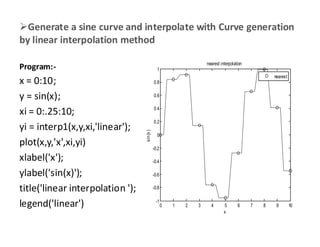
ØGenerate a sinecurve and interpolate with Curve generation
by linear interpolation method
Program:-
x = 0:10;
y = sin(x);
xi = 0:.25:10;
yi = interp1(x,y,xi,'linear');
plot(x,y,'x',xi,yi)
xlabel('x');
ylabel('sin(x)');
title('linear interpolation ');
legend('linear') 0 1 2 3 4 5 6 7 8 9 10
-1
-0.8
-0.6
-0.4
-0.2
0
0.2
0.4
0.6
0.8
1
x
sin
(x
)
nearest interpolation
nearest
46.
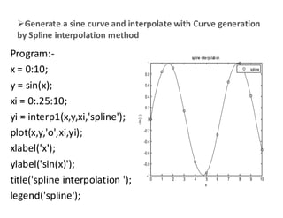
ØGenerate a sinecurve and interpolate with Curve generation
by Spline interpolation method
Program:-
x = 0:10;
y = sin(x);
xi = 0:.25:10;
yi = interp1(x,y,xi,'spline');
plot(x,y,'o',xi,yi);
xlabel('x');
ylabel('sin(x)');
title('spline interpolation ');
legend('spline');
0 1 2 3 4 5 6 7 8 9 10
-1
-0.8
-0.6
-0.4
-0.2
0
0.2
0.4
0.6
0.8
1
x
s
in
(x
)
spline interpolation
spline
47.
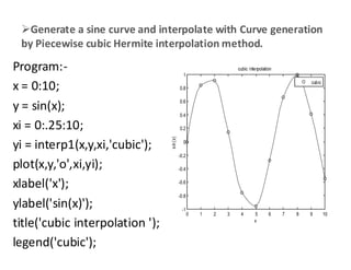
ØGenerate a sinecurve and interpolate with Curve generation
by Piecewise cubic Hermite interpolation method.
Program:-
x = 0:10;
y = sin(x);
xi = 0:.25:10;
yi = interp1(x,y,xi,'cubic');
plot(x,y,'o',xi,yi);
xlabel('x');
ylabel('sin(x)');
title('cubic interpolation ');
legend('cubic');
0 1 2 3 4 5 6 7 8 9 10
-1
-0.8
-0.6
-0.4
-0.2
0
0.2
0.4
0.6
0.8
1
x
s
in
(x)
cubic interpolation
cubic
48.
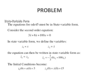
Ø To Findthe solution to the following set of linear equations by Matrix
method:
2x-3y+4z = 5
x+y+4z = 10
3x+4y-2z = 0
Program:-
clc;
clear all;
A=[2 -3 4; 1 1 4; 3 4 -2];
B=*5 10 0+’;
X=inv(A)*B;
(or)
X=AB;
49.
Ø Write programto calculate the average of the given parameters.
Program:
clc;
clear all;
game1 = input('Enter the points scored in the first game ');
game2 = input('Enter the points scored in the second game ');
game3 = input('Enter the points scored in the third game ');
average = (game1+game2+game3)/3
Solution:
Input:
Enter the points scored in the first game
Enter the points scored in the second game
Enter the points scored in the third game
Output:
average =
50.
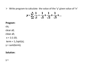
Ø Write programto calculate the value of the ‘y’ given value of ‘n’
Program:
clc;
clear all;
close all;
x = 1:1:10;
term = 1./sqrt(x);
y = sum(term);
Solution:
y =
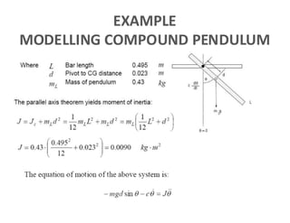
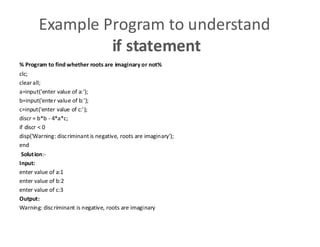
Example Program tounderstand
if statement
% Program to find whether roots are imaginary or not%
clc;
clear all;
a=input('enter value of a:');
b=input('enter value of b:');
c=input('enter value of c:');
discr = b*b - 4*a*c;
if discr < 0
disp('Warning: discriminant is negative, roots are imaginary');
end
Solution:-
Input:
enter value of a:1
enter value of b:2
enter value of c:3
Output:
Warning: discriminant is negative, roots are imaginary
55.
Continued…
Program:-
clc;
clear all;
a=input('enter valueof a:');
b=input('enter value of b:');
c=input('enter value of c:‘);
discr = b*b - 4*a*c;
if discr < 0
disp('Warning: discriminant is negative, roots are imaginary');
else
disp('Roots are real, but may be repeated')
end
Solution:-
Input:
enter value of a:1
enter value of b:3
enter value of c:2
Output:
Roots are real, but may be repeated
56.
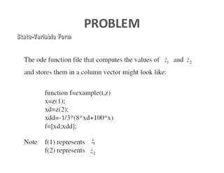
Finding out theroots of quadratic equation ax2+bx+c=0.
Program:-
clear all;
clc;
a=input('Enter valuesfor a:');
b=input('Entervalues forb:');
c=input('Enter values for c:');
delta = b^2 - 4*a*c;
if delta < 0
fprintf('nEquation hasno real roots:nn')
disp(['discriminant = ', num2str(delta)])
elseif delta == 0
fprintf('nEquation hasonereal root:n')
xone = -b/(2*a)
else
fprintf('nEquation hastwo real roots:n')
x(1) = (-b+ sqrt(delta))/(2*a);
x(2) = (-b -sqrt(delta))/(2*a);
fprintf('nFirst root= %10.2ent Second root = %10.2f', x(1),x(2))
end
Algorithm:-
Read in values of a, b, c
Calculate Δ
IF Δ < 0
Printmessage ‘ No real roots’→ Go END
ELSEIF Δ = 0
Printmessage ‘One real root’→ Go END
ELSE
Printmessage ‘Tworeal roots’
END
Solution:-
Input:
Entervalues for a:
Entervalues for b:
Entervalues for c:
Output:
57.
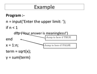
Example
Program :-
n =input(‘Enter the upper limit: ‘);
if n < 1
disp (‘Your answer is meaningless!’)
end
x = 1:n;
term = sqrt(x);
y = sum(term)
Jump to here if TRUE
Jump to here if FALSE
58.
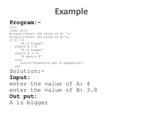
Example
Program:-
clc;
clear all;
A=input(‘enter thevalue of A: ’);
B=input(‘enter the value of B:’);
if A > B
'A is bigger'
elseif A < B
'B is bigger'
elseif A == B
'A equals B'
else
error('Something odd is happening')
end
Solution:-
Input:
enter the value of A: 4
enter the value of B: 3.9
Out put:
A is bigger
59.
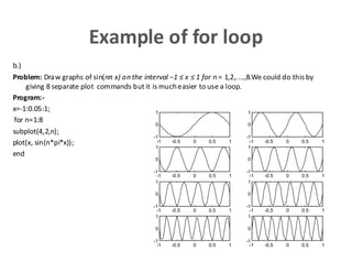
Example of forloop
b.)
Problem: Draw graphs of sin(nπ x) on the interval −1 ≤ x ≤ 1 for n = 1,2,....,8.We could do this by
giving 8 separate plot commands but it is mucheasier to use a loop.
Program:-
x=-1:0.05:1;
for n=1:8
subplot(4,2,n);
plot(x, sin(n*pi*x));
end
-1 -0.5 0 0.5 1
-1
0
1
-1 -0.5 0 0.5 1
-1
0
1
-1 -0.5 0 0.5 1
-1
0
1
-1 -0.5 0 0.5 1
-1
0
1
-1 -0.5 0 0.5 1
-1
0
1
-1 -0.5 0 0.5 1
-1
0
1
-1 -0.5 0 0.5 1
-1
0
1
-1 -0.5 0 0.5 1
-1
0
1
60.
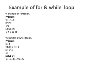
Example of for& while loop
% example of for loop%
Program:-
for ii=1:5
x=ii*ii
end
Solution:
1 4 9 16 25
%example of while loop%
Program:-
x = 1
while x <= 10
x = 3*x
nd
Solution:
x=1 x=3 x= 9 x=27
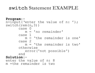
switch Statement EXAMPLE
Program:-
n=input(‘enterthe value of n: ’);
switch(rem(n,3))
case 0
m = 'no remainder'
case 1
m = ‘the remainder is one
case 2
m = ‘the remainder is two
otherwise
error('not possible')
end
Solution:-
enter the value of n: 8
m =the remainder is two
63.
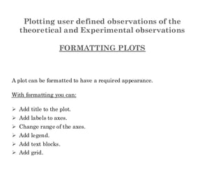
Plotting user definedobservations of the
theoretical and Experimental observations
FORMATTING PLOTS
A plot can be formatted to have a required appearance.
With formatting you can:
Ø Add title to the plot.
Ø Add labels to axes.
Ø Change range of the axes.
Ø Add legend.
Ø Add text blocks.
Ø Add grid.
64.
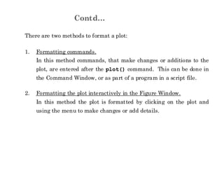
Contd…
There are twomethods to format a plot:
1. Formatting commands.
In this method commands, that make changes or additions to the
plot, are entered after the plot() command. This can be done in
the Command Window, or as part of a program in a script file.
2. Formatting the plot interactively in the Figure Window.
In this method the plot is formatted by clicking on the plot and
using the menu to make changes or add details.
65.
FORMATTING COMMANDS
title(‘string’)
Adds thestring as a title at the top of the plot.
xlabel(‘string’)
Adds the string as a label to the x-axis.
ylabel(‘string’)
Adds the string as a label to the y-axis.
axis([xmin xmax ymin ymax])
Sets the minimum and maximum limits of the x- and y-axes.
66.
FORMATTING COMMANDS
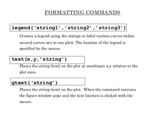
legend(‘string1’,’string2’,’string3’)
Creates alegend using the strings to label various curves (when
several curves are in one plot). The location of the legend is
specified by the mouse.
text(x,y,’string’)
Places the string (text) on the plot at coordinate x,y relative to the
plot axes.
gtext(‘string’)
Places the string (text) on the plot. When the command executes
the figure window pops and the text location is clicked with the
mouse.
67.
Example Program
clc;
clear all;
x=[10:0.1:22];
y=95000./x.^2;
xd=[10:2:22];
yd=[950640 460 340 250 180 140];
plot(x,y,'-','LineWidth',1.0)
hold on
plot(xd,yd,'ro--','linewidth',1.0,'markersize',10)
hold off
xlabel('DISTANCE (cm)')
ylabel('INTENSITY (lux)')
title('fontname{Arial}Light Intensity as a Function of Distance','FontSize',14)
axis([8 24 0 1200])
text(14,700,'Comparison between theory and experiment.','EdgeColor','r','LineWidth',2)
legend('Theory','Experiment',0)
8 10 12 14 16 18 20 22 24
0
200
400
600
800
1000
1200
DISTANCE (cm)
INT
ENSITY
(lux)
Light Intensityas a Function of Distance
Comparison between theory and experiment.
Theory
Experiment
68.
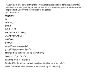
ØConsider a particlemoving in a straight line, and assume that its position is defined by the
equation, where x is expressed in meters and t in seconds. Write a program in MATLAB to
determine the displacement, velocity andacceleration variation with respect to time interval
from 0 to 120 seconds.
Program:-
clc;
clear all;
syms t;
t=0:0.1:120;
x=6.*t.^2-t.^3;
v=12.*t-3.*t.^2;
a=12-6.*t;
plot(t,x);
xlabel(‘time in seconds’);
ylabel(‘displacement in m’);
title(‘displacement of a particle along its motion’);
%plot(t,v);
%xlabel(‘time in seconds’);
%ylabel(‘velocity in m/s’);
%title(‘velocity of a particle in motion’);
%plot(t,a);
%xlabel(‘time in seconds’);
%ylabel(‘acceleration in m/s2’);
%title(‘acceleration of a particle’);
69.
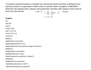
ØA particle movesalong a straight line with variable acceleration. If the displacement is
measured in m, and given by the relation interms of time taken t, as below, determine the
displacement, velocity and acceleration of the particle
S=t3 +2t2+7t+3
Program:-
clc;
clear all;
syms t;
t=0:0.1:120;
x=t.^3+2*t.^2+7.*t+3;
v=3.*t.^2+4.*t+7;
a=6.*t+4;
plot(t,x);
xlabel(‘time in seconds’);
ylabel(‘displacement in m’);
title(‘particle behavior along its motion’);
%plot(t,x,'.'t,v,'o',t,a,'+');
%xlabel(‘time in seconds’);
%ylabel(‘displacement, velocity and acceleration of a particle’);
%title(‘kinematics behavior of a particle along its motion’);
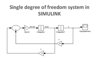
Function of theProgram
function f=programone (t,z)
m=3;
c=8;
k=100;
dzdt=[z(2); -(c/m)*z(2)-(k/m)*z(1)];
76.
Main body ofthe Program
% For a single degree of freedom system in free
vibration
clc;
clear all;
%Enter initial conditions
z0=[5;15];
%Enter time span for solution
tspan=[0 10];
%Call solver
[t,z+=ode45(‘programone',tspan,x0);
%Set up plot
plot(t,z(:,1));
77.
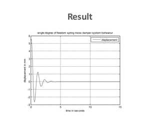
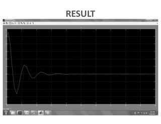
Result
0 5 1015
-3
-2
-1
0
1
2
3
4
5
6
time in seconds
displacement
in
mm
single degree of freedom spring mass damper system behaviour
displacement
78.
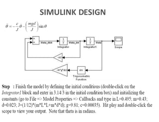
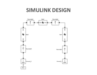
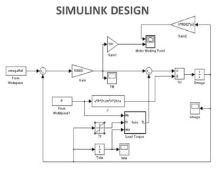
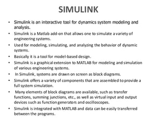
SIMULINK
• Simulink isan interactive tool for dynamics system modeling and
analysis.
• Simulink is a Matlab add-on that allows one to simulate a variety of
engineering systems.
• Used for modeling, simulating, and analyzing the behavior of dynamic
systems.
• Basically it is a tool for model-based design.
• Simulink is a graphical extension to MATLAB for modeling and simulation
of various engineering systems.
• In Simulink, systems are drawn on screen as block diagrams.
• Simulink offers a variety of components that are assembled to provide a
full system simulation.
• Many elements of block diagrams are available, such as transfer
functions, summing junctions, etc., as well as virtual input and output
devices such as function generators and oscilloscopes.
• Simulink is integrated with MATLAB and data can be easily transferred
between the programs.
79.
Simulink
• Simulink canbe used to solve any initial value ODE.
• Modelling/designing dynamic systems including
nonlinear dynamics.
• Modelling/designing control systems including
nonlinear controller plants.
• User creates device model by means of standard blocks
and carries out calculations.
• There are additional block libraries for different scopes
as SimMechanics – mechanical devices modeling,
• SimHydraulics– Hydraulic systems modeling.
81.
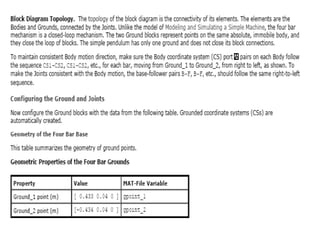
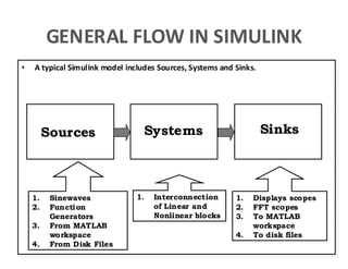
• A typicalSimulink model includes Sources, Systems and Sinks.
Sources Systems Sinks
1. Sinewaves
2. Function
Generators
3. From MATLAB
workspace
4. From Disk Files
1. Interconnection
of Linear and
Nonlinear blocks
1. Displays scopes
2. FFT scopes
3. To MATLAB
workspace
4. To disk files
GENERAL FLOW IN SIMULINK
82.
How to startSimulink
Type Simulink in the
Command window.
Create new model under
file/new/model.
119
83.
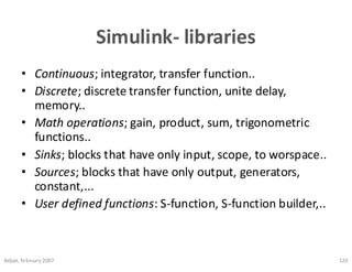
Simulink- libraries
• Continuous;integrator, transfer function..
• Discrete; discrete transfer function, unite delay,
memory..
• Math operations; gain, product, sum, trigonometric
functions..
• Sinks; blocks that have only input, scope, to worspace..
• Sources; blocks that have only output, generators,
constant,...
• User defined functions: S-function, S-function builder,..
Beljak, february 2007 120
84.
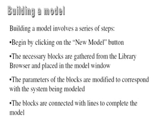
Simulink – creatinga model
• Model is created by choosing the blocks from different
libraries, dragging them to model window and linking
them.
• The parameters of block (shown on picture, sine wave
parameters), can be reached with double click on the
block.
121
An Introduction toSimulink
Configuration Parameters
Simulink is designed to be a front-end tool for
integrating ordinary differential equations
(ODEs).
87.
Connecting blocks
1. Holddown the Control key down.
2. Click on the “source” icon.
3. Click on the “sink” icon.
4. Press the left mouse key to make the
connection.
88.
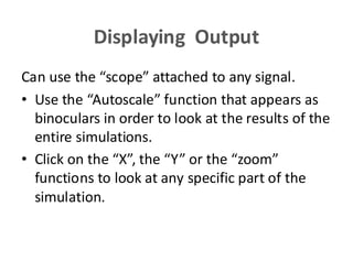
Displaying Output
Can usethe “scope” attached to any signal.
• Use the “ utoscale” function that appears as
binoculars in order to look at the results of the
entire simulations.
• Click on the “X”, the “Y” or the “zoom”
functions to look at any specific part of the
simulation.
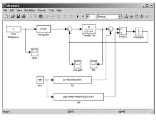
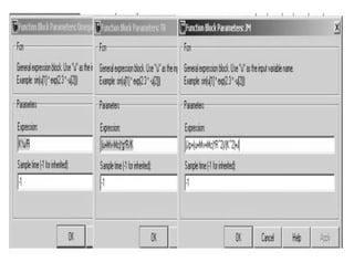
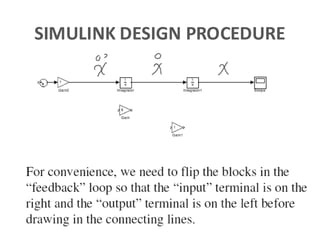
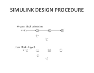
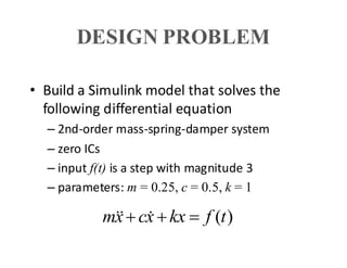
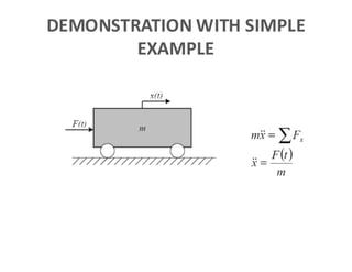
DESIGN PROBLEM
• Builda Simulink model that solves the
following differential equation
– 2nd-order mass-spring-damper system
– zero ICs
– input f(t) is a step with magnitude 3
– parameters: m = 0.25, c = 0.5, k = 1
)
(t
f
kx
x
c
x
m =
+
+
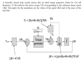
CONVERSIONS IN MATLAB
Transferfunction to state space [A,B,C,D]=tf2ss([num],[den]);
State-space to transfer function [num,den]=ss2tf(A,B,C,D);
Transfer function to zero/poles [z,p,k]=tf2zp([num],[den]);
Zero/poles to transfer function [num,den]=zp2tf(z,p,k);
State space to zero/poles [z,p,k]=ss2zp(A,B,C,D,iu);
Zero/poles to state space [A,B,C,D]=zp2ss(z,p,k);
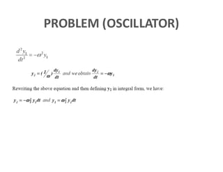
REAL TIME CHALLENGINGPROBLEM
Landing gear Suspension schematic
Ys
Yin
Yo
M in
s
o y
y
y
y -
-
=
( )
dt
dy
dt
dy
dt
y
y
y
d
dt
dy in
o
in
s
o
-
=
-
-
=
128.
Force balance
M
Mg FsFc
å -
-
-
=
= s
c
y F
F
Mg
Ma
F
s
c
o
F
F
Mg
dt
y
d
M -
-
-
=
2
2
129.
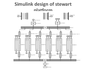
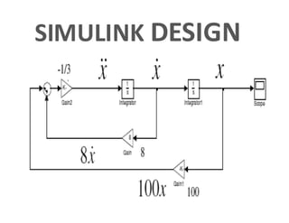
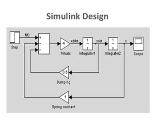
Simulink design
ò ÷
ø
ö
ç
è
æ
-
-
-
=dt
M
F
M
F
g
v s
c
dt
v
yo ò
=
)
( 0 s
in
s y
y
y
k
F -
-
=
ú
û
ù
ê
ë
é
-
=
dt
dy
dt
dy
C
F in
o
c
Yin
Scope
0
Mg
1
Ks
1
s
Integrator2
1
s
Integrator1
du/dt
Derivative
.5
C
.5
1/M
Mv
v =dYo/dt
v =dYo/dt Y0
Fs
Mg
Yo-Y in
dYin/dt Fc
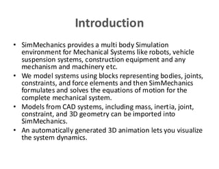
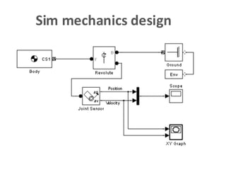
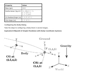
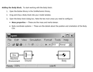
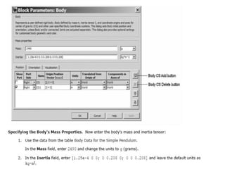
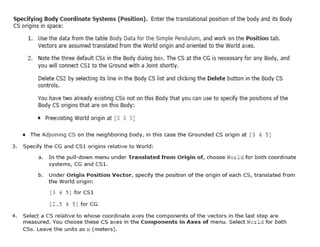
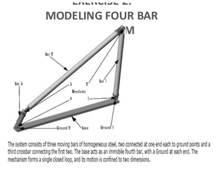
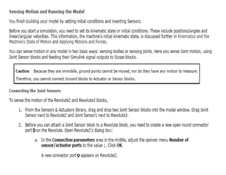
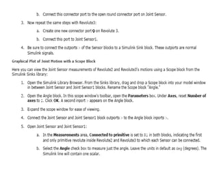
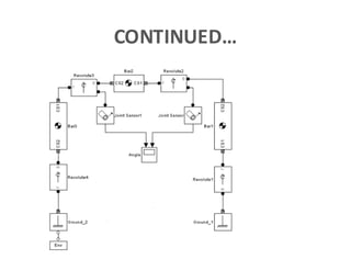
Introduction
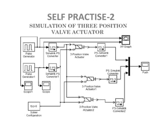
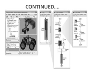
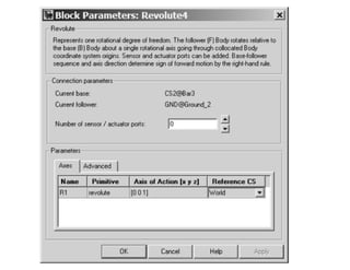
• SimMechanics providesa multi body Simulation
environment for Mechanical Systems like robots, vehicle
suspension systems, construction equipment and any
mechanism and machinery etc.
• We model systems using blocks representing bodies, joints,
constraints, and force elements and then SimMechanics
formulates and solves the equations of motion for the
complete mechanical system.
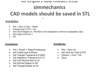
• Models from CAD systems, including mass, inertia, joint,
constraint, and 3D geometry can be imported into
SimMechanics.
• An automatically generated 3D animation lets you visualize
the system dynamics.
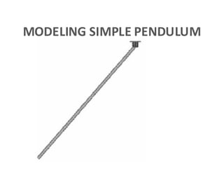
172.
NOT JUST NIMTION….!
IT DOES LOT OF BACK GROUND
COMPUTATIONAL MECHANICS
WORK
OPEN WEB RESOURCES
•Mathworks Information
• Mathworks: http://www.mathworks.com
• Mathworks Central: http://www.mathworks.com/matlabcentral
• http://www.mathworks.com/applications/controldesign/
• http://www.mathworks.com/academia/student_center/tutorials/l
aunchpad.html
• Matlab Demonstrations
• Matlab Overview: A demonstration of the Capabilities of Matlab
http://www.mathworks.com/cmspro/online/4843/req.html?13616
• Numerical Computing with Matlab
http://www.mathworks.com/cmspro/online/7589/req.html?16880
• Select Help-Demos in Matlab
269.
OPEN WEB RESOURCES
•Matlab Help
• Select “Help” in Matlab. Extensive help about Matlab, Simulink and toolboxes
• Matlab Homework Helper
http://www.mathworks.com/academia/student_center/homework/
• Newsgroup: comp.soft-sys.matlab
• Matlab/Simulink student version (program and book ~£50)
http://www.mathworks.com/academia/student_center
• Other Matlab and Simulink Books
• Mastering Matlab 6, Hanselman & Littlefield, Prentice Hall
• Mastering Simulink 4, Dabney & Harman, Prentice Hall
• Matlab and Simulink Student Version Release 14
• lots more on mathworks, amazon, …. It is important to have one reference book.
![Matrixes and vectors
• x = [1,2,3] , vector-row,
• y=[1;2;3], vector-column,
• x=0:0.1:0.8 , vector x=[0,0.1,0.2,0.3....0.8],
• A = [1,3,5;5,6,7;8,9,10], matrix,
• A(1,2), element of matrix, 1. row, 2. column,
• A(:,2), second column of matrix,
• A(1,:), first row of matrix ,
• C=[A;[10,20,30]] matrix with additional row,
• B=A(2:3,1:2), part of matrix,
• x’, transpose.
46](https://image.slidesharecdn.com/lecturenotesmatlab-250624170418-8ac1b522/85/Notes-and-guide-for-matlab-coding-and-excersie-9-320.jpg)
![Solving Nonlinear Equations by
Function
nle.m (function of the program)
function f = nle(x)
f(1) = x(1)-4*x(1)*x(1)-x(1)*x(2);
f(2) = 2*x(2)-x(2)*x(2)+3*x(1)*x(2);
Main body of the Program:-
x0 = [1 1]';
x = fsolve('nle', x0)
Solution of the program:-
x =
0.2500
0.0000](https://image.slidesharecdn.com/lecturenotesmatlab-250624170418-8ac1b522/85/Notes-and-guide-for-matlab-coding-and-excersie-14-320.jpg)
![ØPlot of the sine function from limits of 0 to (2* pi).
Program:-
clear all; % clear all variables
clc; % clear screen
N=30;
h=pi/N;
x=0:h:(2*pi);
y=sin(x);
plot(x,y)
xlabel('x')
ylabel('sin(x')
title('Graph of sine function in 0 to (2*pi) range')
0 1 2 3 4 5 6 7
-1
-0.8
-0.6
-0.4
-0.2
0
0.2
0.4
0.6
0.8
1
x
sin(x)
Graph of sine function in 0 to (2*pi) range
sin(x)
Hint: - Direct plotting of curves can be done by ‘fplot’ command also
Syntax: fplot (‘function’, *lower limit, upper limit)
fplot ('x*cos(x)',[0, 10*pi]);](https://image.slidesharecdn.com/lecturenotesmatlab-250624170418-8ac1b522/85/Notes-and-guide-for-matlab-coding-and-excersie-32-320.jpg)
![Ø To plot the function y(x)= -3*x+4 from limits -1 to 2.
Program:-
clc;
clear all;
x=-1:1:2;
y=-3*x+4;
figure
plot(x,y)
xlabel('x')
ylabel('y=f(x)')
grid on
title('plot of function f_1(x)');
legend('f_1(x)');
axis([-2 4 -2 12])
-2 -1 0 1 2 3 4
-2
0
2
4
6
8
10
12
x
y=f(x)
plot of function f1
(x)
f1
(x)](https://image.slidesharecdn.com/lecturenotesmatlab-250624170418-8ac1b522/85/Notes-and-guide-for-matlab-coding-and-excersie-33-320.jpg)
![ØComparing multiple plots in single window for example
y1 = 2 cos(x), y2 = cos(x), and y3 =0.5* cos(x), in the interval 0≤ x≤ (2*pi)
Program:-
x = 0:pi/100:2*pi;
y1 = 2*cos(x);
y2 = cos(x);
y3 = 0.5*cos(x);
plot(x,y1,'--',x,y2,'-',x,y3,':');
xlabel('0 leq x leq 2pi');
ylabel('Cosine functions');
legend('2*cos(x)','cos(x)','0.5*cos(x)');
title('Typical example of multiple plots');
axis([0 2*pi -3 3]);
0 1 2 3 4 5 6
-3
-2
-1
0
1
2
3
0 £ x £ 2p
Cosine
func
tions
Typical example of multiple plots
2*cos(x)
cos (x)
0.5*cos(x)](https://image.slidesharecdn.com/lecturenotesmatlab-250624170418-8ac1b522/85/Notes-and-guide-for-matlab-coding-and-excersie-35-320.jpg)
![ØTo plot the curve of exponential of x and sin(x) in a single
window
Program:-
clc;
clear all;
x=0:.1:2*pi;
y=sin(x);
plot(x,y);
grid on;
hold on;
plot(x, exp(-x), 'r:*');
axis([0 2*pi 0 1]);
title('2-D Plot');
xlabel('Time');
ylabel('Sin(t) ');
text(pi/3, sin(pi/3), '<--sin(pi/3) ');
legend('Sine Wave','Decaying Exponential');
0 1 2 3 4 5 6
0
0.1
0.2
0.3
0.4
0.5
0.6
0.7
0.8
0.9
1
2-D Plot
Time
Sin
(t)
<--sin(p/3)
Sine Wave
Decaying Exponential](https://image.slidesharecdn.com/lecturenotesmatlab-250624170418-8ac1b522/85/Notes-and-guide-for-matlab-coding-and-excersie-36-320.jpg)
![ØFor the given data plot the variation of x with y.
Program:
clc;
Clear all;
x=[1 2 3 5 7 7.5 8 10];
y=[2 6.5 7 7 5.5 4 6 8];
plot(x, y)
x
y
1 2 3 5 7 7.5 8
6.5 7 7 5.5 4 6 8
10
2](https://image.slidesharecdn.com/lecturenotesmatlab-250624170418-8ac1b522/85/Notes-and-guide-for-matlab-coding-and-excersie-38-320.jpg)
![Ø For the given data plot the variation of x with y.
Program:
clc;
Clear all;
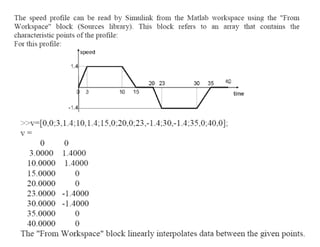
year = [1988:1:1994];
sales = [127, 130, 136, 145, 158, 178, 211];
plot(year, sales,'--r*')
Year
Sales (M)
1988 1989 1990 1991 1992 1993 1994
127 130 136 145 158 178 211](https://image.slidesharecdn.com/lecturenotesmatlab-250624170418-8ac1b522/85/Notes-and-guide-for-matlab-coding-and-excersie-39-320.jpg)
![Ø Plot the surface defined by the function
f(x,y)= (x-3)2 – (y-2)2 on the domain -2 ≤ x ≤ 4 and 1 ≤ y ≤ 3.
Program:-
clc;
clear all;
[X,Y] = meshgrid(-2:0.2:4,1:0.2:3);
Z = (X-3).^2 - (Y-2).^2;
mesh(X,Y,Z);
xlabel('x');
ylabel('y');
-2
0
2
4
1
1.5
2
2.5
3
-5
0
5
10
15
20
25
x
y](https://image.slidesharecdn.com/lecturenotesmatlab-250624170418-8ac1b522/85/Notes-and-guide-for-matlab-coding-and-excersie-42-320.jpg)
![Ø To Find the solution to the following set of linear equations by Matrix
method:
2x-3y+4z = 5
x+y+4z = 10
3x+4y-2z = 0
Program:-
clc;
clear all;
A=[2 -3 4; 1 1 4; 3 4 -2];
B=*5 10 0+’;
X=inv(A)*B;
(or)
X=AB;](https://image.slidesharecdn.com/lecturenotesmatlab-250624170418-8ac1b522/85/Notes-and-guide-for-matlab-coding-and-excersie-48-320.jpg)

![Finding out the roots of quadratic equation ax2+bx+c=0.
Program:-
clear all;
clc;
a=input('Enter valuesfor a:');
b=input('Entervalues forb:');
c=input('Enter values for c:');
delta = b^2 - 4*a*c;
if delta < 0
fprintf('nEquation hasno real roots:nn')
disp(['discriminant = ', num2str(delta)])
elseif delta == 0
fprintf('nEquation hasonereal root:n')
xone = -b/(2*a)
else
fprintf('nEquation hastwo real roots:n')
x(1) = (-b+ sqrt(delta))/(2*a);
x(2) = (-b -sqrt(delta))/(2*a);
fprintf('nFirst root= %10.2ent Second root = %10.2f', x(1),x(2))
end
Algorithm:-
Read in values of a, b, c
Calculate Δ
IF Δ < 0
Printmessage ‘ No real roots’→ Go END
ELSEIF Δ = 0
Printmessage ‘One real root’→ Go END
ELSE
Printmessage ‘Tworeal roots’
END
Solution:-
Input:
Entervalues for a:
Entervalues for b:
Entervalues for c:
Output:](https://image.slidesharecdn.com/lecturenotesmatlab-250624170418-8ac1b522/85/Notes-and-guide-for-matlab-coding-and-excersie-56-320.jpg)
![While Loop EXAMPLES
Program:-
S = 1;
n = 1;
while S+(n+1)^2 < 100
n = n+1;
S = S + n^2;
end
Solution:-
[n,S] = 6 91](https://image.slidesharecdn.com/lecturenotesmatlab-250624170418-8ac1b522/85/Notes-and-guide-for-matlab-coding-and-excersie-61-320.jpg)
![FORMATTING COMMANDS
title(‘string’)
Adds the string as a title at the top of the plot.
xlabel(‘string’)
Adds the string as a label to the x-axis.
ylabel(‘string’)
Adds the string as a label to the y-axis.
axis([xmin xmax ymin ymax])
Sets the minimum and maximum limits of the x- and y-axes.](https://image.slidesharecdn.com/lecturenotesmatlab-250624170418-8ac1b522/85/Notes-and-guide-for-matlab-coding-and-excersie-65-320.jpg)
![Example Program
clc;
clear all;
x=[10:0.1:22];
y=95000./x.^2;
xd=[10:2:22];
yd=[950 640 460 340 250 180 140];
plot(x,y,'-','LineWidth',1.0)
hold on
plot(xd,yd,'ro--','linewidth',1.0,'markersize',10)
hold off
xlabel('DISTANCE (cm)')
ylabel('INTENSITY (lux)')
title('fontname{Arial}Light Intensity as a Function of Distance','FontSize',14)
axis([8 24 0 1200])
text(14,700,'Comparison between theory and experiment.','EdgeColor','r','LineWidth',2)
legend('Theory','Experiment',0)
8 10 12 14 16 18 20 22 24
0
200
400
600
800
1000
1200
DISTANCE (cm)
INT
ENSITY
(lux)
Light Intensityas a Function of Distance
Comparison between theory and experiment.
Theory
Experiment](https://image.slidesharecdn.com/lecturenotesmatlab-250624170418-8ac1b522/85/Notes-and-guide-for-matlab-coding-and-excersie-67-320.jpg)
![Function of the Program
function f=programone (t,z)
m=3;
c=8;
k=100;
dzdt=[z(2); -(c/m)*z(2)-(k/m)*z(1)];](https://image.slidesharecdn.com/lecturenotesmatlab-250624170418-8ac1b522/85/Notes-and-guide-for-matlab-coding-and-excersie-75-320.jpg)
![Main body of the Program
% For a single degree of freedom system in free
vibration
clc;
clear all;
%Enter initial conditions
z0=[5;15];
%Enter time span for solution
tspan=[0 10];
%Call solver
[t,z+=ode45(‘programone',tspan,x0);
%Set up plot
plot(t,z(:,1));](https://image.slidesharecdn.com/lecturenotesmatlab-250624170418-8ac1b522/85/Notes-and-guide-for-matlab-coding-and-excersie-76-320.jpg)


![CONVERSIONS IN MATLAB
Transfer function to state space [A,B,C,D]=tf2ss([num],[den]);
State-space to transfer function [num,den]=ss2tf(A,B,C,D);
Transfer function to zero/poles [z,p,k]=tf2zp([num],[den]);
Zero/poles to transfer function [num,den]=zp2tf(z,p,k);
State space to zero/poles [z,p,k]=ss2zp(A,B,C,D,iu);
Zero/poles to state space [A,B,C,D]=zp2ss(z,p,k);](https://image.slidesharecdn.com/lecturenotesmatlab-250624170418-8ac1b522/85/Notes-and-guide-for-matlab-coding-and-excersie-104-320.jpg)